Today, we are going to explore the exciting world of Perfect Competition. This concept is crucial for understanding how markets work and how firms make decisions. Let’s break it down step by step with simple everyday examples and some real-world case studies.
Introduction
Perfect Competition is an idealized market structure where many firms offer a homogeneous product, and no single firm can influence the market price. This market structure is characterized by several key features that ensure efficiency in the allocation of resources.
Characteristics of Perfect Competition
1. Large Number of Buyers and Sellers
- Explanation: In a perfectly competitive market, there are so many buyers and sellers that no single buyer or seller can influence the market price. Each participant is a price taker, meaning they accept the market price as given.
- Example: Think of the agricultural markets in Punjab, Pakistan, where numerous farmers sell wheat. No single farmer can set the price of wheat; they must accept the prevailing market price.
2. Homogeneous Products
- Explanation: The products offered by different sellers are identical in the eyes of consumers. There are no brand differences or quality variations.
- Example: Rice sold in Bangladesh markets is often seen as homogeneous, with each seller offering the same type of rice as their competitors.
3. Free Entry and Exit
- Explanation: Firms can freely enter or exit the market without significant barriers. This ensures that if firms are making supernormal profits, new firms will enter the market, increasing supply and reducing prices until only normal profits are made.
- Example: Small shops selling everyday items in Karachi, Pakistan, can easily start or shut down their businesses based on profitability without facing high entry or exit costs.
4. Perfect Information
- Explanation: All participants in the market have complete and accurate information about prices, products, and market conditions. This ensures that no one has an advantage over others due to better information.
- Example: In modern stock markets like the Bombay Stock Exchange, information about stock prices and company performance is readily available to all investors, ensuring a level playing field.
5. Perfect Mobility of Factors of Production
- Explanation: Resources such as labor and capital can move freely in and out of the industry. There are no restrictions on the mobility of factors of production.
- Example: Workers in the garment industry in Dhaka, Bangladesh, can switch to other industries or jobs if they find better opportunities, ensuring that labor is allocated where it is most needed.
6. No Government Intervention
- Explanation: There is no government interference in the market in the form of taxes, subsidies, or regulations that could distort the natural market equilibrium.
- Example: In a theoretical perfectly competitive market, there would be no tariffs or subsidies affecting the price of imported or exported goods.
Significance of Perfect Competition
Efficiency:
- Productive Efficiency: Firms produce at the lowest possible cost. This is achieved when firms operate at the minimum point of their long-run average cost curve.
- Allocative Efficiency: Resources are allocated to produce the mix of goods and services most desired by society. This occurs when the price of the good equals the marginal cost of production (P = MC).
Price and Output Determination:
- In the short run, firms in a perfectly competitive market will produce up to the point where marginal cost equals marginal revenue (MC = MR).
- In the long run, the entry and exit of firms ensure that all firms in the market make normal profits, and prices stabilize at a level where firms earn zero economic profit.
Output Decisions in Perfectly Competitive Market
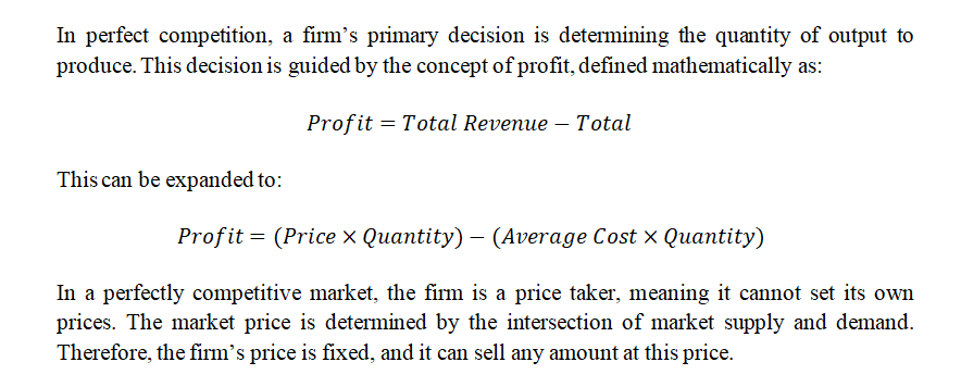
Market Price and Demand
In perfect competition, the firm faces a perfectly elastic demand curve. This means that the firm can sell any quantity of its product at the prevailing market price. For instance, if a small farmer produces raspberries and the market price is $4 per pack, the farmer can sell any number of packs at this price.
Determining Profit: Total Revenue vs. Total Cost
We analyze the relationship between total revenue and total cost to find the optimal production quantity.
- Total Revenue (TR) is calculated as:
TR=Price x Quantity
- Total Cost (TC) includes both fixed and variable costs. The TC curve starts at the fixed cost level and rises with output.
Graphical Analysis
1. Total Revenue and Total Cost Approach
- Horizontal Axis (Quantity): Number of packs of raspberries produced.
- Vertical Axis (Cost/Revenue): Measured in dollars.
- Total Revenue Curve: A straight line, because the price is constant.
Total Cost Curve: Starts at the fixed cost level and slopes upwards, steepening due to diminishing marginal returns.
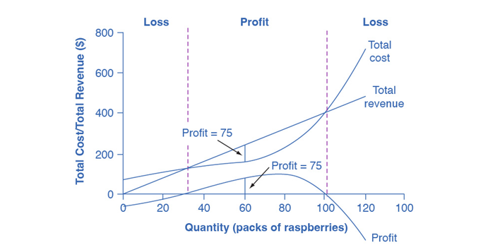
Example Data:
| Quantity (Q) | Total Cost (TC) | Total Revenue (TR) | Profit |
| 0 | $62 | $0 | -$62 |
| 10 | $90 | $40 | -$50 |
| 20 | $110 | $80 | -$30 |
| 30 | $126 | $120 | -$6 |
| 40 | $138 | $160 | $22 |
| 50 | $150 | $200 | $50 |
| 60 | $165 | $240 | $75 |
| 70 | $190 | $280 | $90 |
| 80 | $230 | $320 | $90 |
| 90 | $296 | $360 | $64 |
| 100 | $400 | $400 | $0 |
| 110 | $550 | $440 | -$110 |
| 120 | $715 | $480 | -$235 |
Profit Maximization
The goal is to determine the output level where profit is maximized, which is where the vertical gap between total revenue and total cost is greatest.
At Q=60 packs
Total Revenue = $240
Total Cost = $165.
Profit = $75.
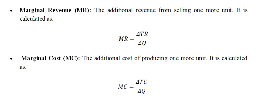
2. Marginal Analysis: Marginal Revenue (MR) and Marginal Cost (MC) Approach
Graphical Analysis: Marginal Revenue and Marginal Cost
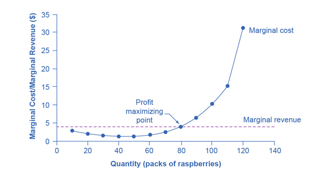
- Horizontal Axis (Quantity): Number of packs of raspberries produced.
- Vertical Axis (Cost/Revenue): Measured in dollars.
- Marginal Revenue Curve: A horizontal line at the market price, $4. This is because the price is constant in perfect competition.
- Marginal Cost Curve: Initially downward-sloping due to increasing marginal returns at low production levels, then upward-sloping due to diminishing marginal returns.
Example Data:
| Quantity (Q) | Total Cost (TC) | Marginal Cost (MC) | Total Revenue (TR) | Marginal Revenue (MR) | Profit |
| 0 | $62 | – | $0 | $4 | -$62 |
| 10 | $90 | $2.80 | $40 | $4 | -$50 |
| 20 | $110 | $2.00 | $80 | $4 | -$30 |
| 30 | $126 | $1.60 | $120 | $4 | -$6 |
| 40 | $138 | $1.20 | $160 | $4 | $22 |
| 50 | $150 | $1.20 | $200 | $4 | $50 |
| 60 | $165 | $1.50 | $240 | $4 | $75 |
| 70 | $190 | $2.50 | $280 | $4 | $90 |
| 80 | $230 | $4.00 | $320 | $4 | $90 |
| 90 | $296 | $6.60 | $360 | $4 | $64 |
| 100 | $400 | $10.40 | $400 | $4 | $0 |
| 110 | $550 | $15.00 | $440 | $4 | -$110 |
| 120 | $715 | $16.50 | $480 | $4 | -$235 |
Profit-Maximizing Output
The profit-maximizing output occurs where MR = MC.
Detailed Analysis:
- At Q=80
- MR = $4 and MC = $4.
- This is the point where profit is maximized.
Practical Example:
- If MR > MC (e.g., at Q = 60 packs), increasing production raises profit.
- If MC > MR (e.g., at Q = 100 packs), reducing production increases profit.
Summary
The profit-maximizing rule for the perfectly competitive market: Produce at the quantity where MR = MC or where P = MC.
In summary, a perfectly competitive firm maximizes profit by producing at the output level where the marginal cost equals the marginal revenue. This ensures that the firm is operating efficiently, maximizing its profit, and not producing beyond the point where costs exceed revenues.
3. Average Cost Curve Approach
In perfect competition, the condition MR=MC maximizes profit, but it doesn’t guarantee positive economic profit. The actual economic profit depends on the relationship between the market price and the average total cost (ATC) of production.
Market Price and Average Total Cost
Economic Profit:
- Occurs when the market price is higher than the ATC.
- The firm earns positive profit margins.
Economic Loss:
Happens when the market price is lower than the ATC.
The firm incurs losses but might continue operating to cover some of its fixed costs.
Break-Even Point:
When the market price equals the ATC.
The firm earns zero economic profit.
Graphical Scenarios: Detailed Breakdown
Let’s elaborate on the three scenarios using graphical representations:
a. Section a. Profit Scenario (Price above ATC)
- Market Price ($5): The market price is represented by a horizontal line at $5.
- Marginal Cost (MC) and Average Cost (AC) Curves: The MC curve intersects the U-shaped AC curve at its minimum point.
- Profit-Maximizing Output: The intersection of P=MRP = MRP=MR and MCMCMC occurs at point E, where the quantity is 85 packs.
- Positive Profits:
- Total Revenue (TR): Represented by the rectangle from the origin to 85 packs, up to the price of $5, and back to the origin.
- Total Cost (TC): Shown by the rectangle from the origin to 85 packs, up to the point where it intersects the AC curve (point C), over to the vertical axis, and down to the origin.
- Profit: The area of the blue-shaded rectangle, which is the difference between TR and TC.
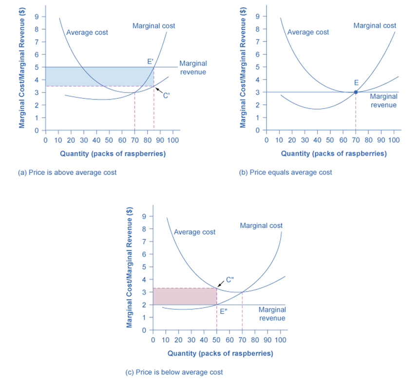

b. Section b. Break-Even Scenario (Price Equals ATC)
- Market Price ($3): The market price is represented by a horizontal line at $3.
- Profit-Maximizing Output: The intersection of P=MRP = MRP=MR and MCMCMC occurs at point E, where the quantity is 75 packs.
- Break-Even:
- Total Revenue (TR) and Total Cost (TC): Both are represented by the same rectangle, as the price equals the average cost.

c. Section c: Loss Scenario (Price below ATC)
- Market Price ($2): The market price is represented by a horizontal line at $2.
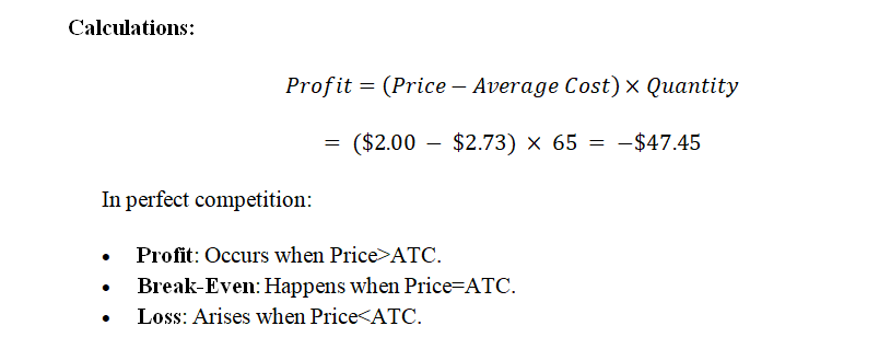
- Profit-Maximizing Output: The intersection of P=MR and MC occurs at point E, where the quantity is 65 packs.
- Negative Profits:
- Total Revenue (TR): Represented by the rectangle from the origin to 65 packs, up to the price of $2, and back to the origin.
- Total Cost (TC): Shown by the rectangle from the origin to 65 packs, up to the point where it intersects the AC curve (point C), over to the vertical axis, and down to the origin.
- Loss: The area of the red-shaded rectangle, which is the difference between TR and TC.
Key Points
- A firm continues to operate with losses in the short run to cover some fixed costs.
- Optimal output is where MR=MC, but economic profit depends on the price relative to ATC.
| If… | Then… |
| Price > ATC | Firm earns a profit |
| Price = ATC | Firm breaks even |
| Price < ATC | Firm incurs a loss |
Summary
In summary, whether a firm earns a profit, breaks even, or incurs a loss in perfect competition is determined by the relationship between the market price and the average total cost. The intersection of the price line with the marginal cost curve at various levels relative to the ATC curve illustrates these scenarios clearly.
Exit or Shutdown Decision of a Perfectly Competitive Firm
When a firm is experiencing losses, the decision to shut down or continue operating depends on its ability to cover variable costs, not just fixed costs.
Understanding Fixed and Variable Costs
Fixed Costs (FC):
Incurred regardless of production level.
Examples: Rent, equipment leases.
Variable Costs (VC):
Change with production level.
Examples: Wages for labor, raw materials.
Shutting down eliminates variable costs but fixed costs remain to bear as a loss.
Numerical Example: a Bakery’s Shutdown Decision
Suppose a bakery enters the market bearing these costs
Fixed Costs: $5,000 per month (rent, equipment depreciation, etc.)
Variable Costs: Cost per loaf of bread is $2.00
Market Prices: Vary throughout the month. Here are the prices and corresponding data:
- Price = $3.50 per loaf
- Price = $2.50 per loaf
- Price = $1.50 per loaf
| Scenario | Price per Loaf | Quantity Produced (loaves) | Total Revenue | Variable Cost | Fixed Cost | Total Cost | Profit/Loss | Decision |
| 1 | $3.50 | 1,000 | $3,500 | $2,000 | $5,000 | $7,000 | -$3,500 | Continue |
| 2 | $2.50 | 900 | $2,250 | $1,800 | $5,000 | $6,800 | -$4,550 | Continue |
| 3 | $1.50 | 600 | $900 | $1,200 | $5,000 | $6,200 | -$5,300 | Shut Down |
Costs and Revenues
Let’s determine whether the bakery should continue producing bread or shut down under different market prices.
Scenario 1: Price = $3.50 per loaf
- Quantity Produced: 1,000 loaves (based on profit-maximizing condition, where MR = MC)
- Total Revenue: Price × Quantity = $3.50 × 1,000 = $3,500
- Variable Cost: Variable Cost per loaf × Quantity = $2.00 × 1,000 = $2,000
- Total Cost: Fixed Costs + Variable Costs = $5,000 + $2,000 = $7,000
- Profit Calculation: Profit=Total Revenue−Total Cost=$3,500−$7,000=−$3,500
- Decision: Since the bakery is making a loss, it must decide whether to continue producing or shut down.
Scenario 2: Price = $2.50 per loaf
- Quantity Produced: 900 loaves (based on profit-maximizing condition, where MR = MC)
- Total Revenue: Price × Quantity = $2.50 × 900 = $2,250
- Variable Cost: Variable Cost per loaf × Quantity = $2.00 × 900 = $1,800
- Total Cost: Fixed Costs + Variable Costs = $5,000 + $1,800 = $6,800
- Profit Calculation: Profit=Total Revenue−Total Cost=$2,250−$6,800=−$4,550
- Decision: The bakery is still making a loss, and must decide on continuing production or shutting down.
Scenario 3: Price = $1.50 per loaf
- Quantity Produced: 600 loaves (based on profit-maximizing condition, where MR = MC)
- Total Revenue: Price × Quantity = $1.50 × 600 = $900
- Variable Cost: Variable Cost per loaf × Quantity = $2.00 × 600 = $1,200
- Total Cost: Fixed Costs + Variable Costs = $5,000 + $1,200 = $6,200
- Profit Calculation: Profit=Total Revenue−Total Cost=$900−$6,200=−$5,300
- Decision: The bakery’s loss is significant, and it must decide whether to shut down or continue production.
Shutdown Point Analysis
- Average Variable Cost (AVC) at Different Quantities: (VC/Q)
- At 1,000 loaves, AVC = $2.00 (per loaf)
- At 900 loaves, AVC = $2.00 (per loaf)
- At 600 loaves, AVC = $2.00 (per loaf)
- Shutdown Point: The shutdown point is where the price equals the minimum average variable cost. Here, it is $2.00 per loaf.
Hence
- Scenario 1: Price = $3.50 > AVC ($2.00) → Continue Production
- Scenario 2: Price = $2.50 > AVC ($2.00) → Continue Production
- Scenario 3: Price = $1.50 < AVC ($2.00) → Shut Down
Summary
- Price = $3.50: Bakery should continue producing, as price covers average variable costs and contributes to fixed costs.
- Price = $2.50: Bakery should continue producing, as price is above AVC.
- Price = $1.50: Bakery should shut down, as price is below AVC, making variable costs unpayable.
This example demonstrates how the bakery evaluates its decision to stay in business or shut down, based on the relationship between market price and average variable cost.
Graphical Illustration of Shutdown Point
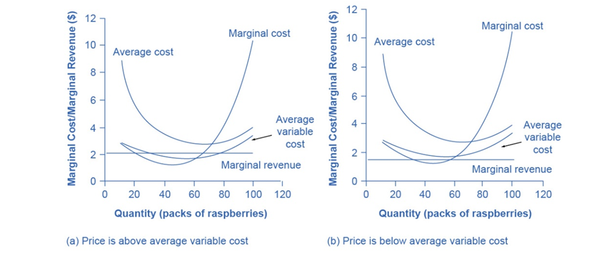
Section 1: Operation Despite Losses
- Market Price ($2): Horizontal line at $2.
- Output Level: Producing 65 packs.
- Loss Calculation:
- Total Revenue:
- Total Cost:
- Loss:
- Fixed Costs: $62
- Decision: Continue operating to minimize losses as price is above average variable cost (AVC).
Section 2: Shutdown Decision
- Market Price ($1.50): Horizontal line at $1.50.
- Output Level: Producing 60 packs.
- Loss Calculation:
- Total Revenue: 60×1.50=$90
- Total Cost: 60×2.75=$165
- Loss:
- Fixed Costs: $62
- Decision: Shut down as operating increases losses beyond fixed costs.
Summary of Scenarios
- If Price > AVC: Continue operating to cover some fixed costs.
- If Price < AVC: Shut down as operating increases losses.
Key Points from Graphs and Table
- Shutdown Point: Price below minimum AVC leads to shutdown.
- Operation Point: Price above AVC leads to continued operation despite losses.
Hence in perfect competition:
- Above AVC: Operate to minimize losses.
- Below AVC: Shut down immediately.
Understanding the shutdown point helps firms make informed decisions about continuing operations versus shutting down in the short run.
Short-Run Outcomes for Perfectly Competitive Firms
Let’s consider a hypothetical example to illustrate these concepts in more detail. Imagine a firm producing handmade candles. The firm’s cost structure includes both fixed and variable costs, and it operates in a perfectly competitive market where it accepts the market price as given.
| Scenario | Market Price per Candle | Break-Even Point | Shutdown Point | Quantity Produced (candles) | Total Revenue | Total Variable Cost | Total Fixed Cost | Total Cost | Profit/Loss | Decision |
| 1 | $10 | $7 | $4 | 100 | $1,000 | $200 | $500 | $700 | $300 | Continue |
| 2 | $7 | $7 | $4 | 100 | $700 | $200 | $500 | $700 | $0 | Continue |
| 3 | $5 | $7 | $4 | 100 | $500 | $200 | $500 | $700 | -$200 | Continue |
| 4 | $3 | $7 | $4 | 0 | $0 | $0 | $500 | $500 | -$500 | Shut Down |
Cost Curves Breakdown:
- Average Cost (AC): This curve represents the total cost (fixed + variable) per unit of output.
- Average Variable Cost (AVC): This curve shows the variable cost per unit of output.
- Marginal Cost (MC): This curve indicates the additional cost of producing one more unit of output.
Profit-Maximizing Output
To maximize profit, the candle-making firm produces where P = MR = MC. Let’s consider three possible scenarios based on the market price:
Price Above Break-Even Point (Profits):
Scenario: The market price is $10 per candle.
Break-Even Point: The MC curve intersects the AC curve at a cost of $7 per candle.
Decision: Since $10 (price) > $7 (average cost), the firm earns a profit.
Profit Calculation: Profit=(Price−AC)×Quantity
If the firm produces 100 candles: Profit= (10−7) ×100=$300
Price at Break-Even Point (Zero Profit):
Scenario: The market price is $7 per candle.
Break-Even Point: The MC curve intersects the AC curve at a cost of $7 per candle.
Decision: Since $7 (price) = $7 (average cost), the firm earns zero profit.
Profit Calculation:
Price Below Break-Even Point but Above Shutdown Point (Operational Losses):
Scenario: The market price is $5 per candle.
Shutdown Point: The MC curve intersects the AVC curve at a cost of $4 per candle.
Decision: Since $5 (price) > $4 (average variable cost) but $5 < $7 (average cost), the firm incurs losses but continues to operate.
Loss Calculation
Price Below Shutdown Point (Shutdown):
Scenario: The market price is $3 per candle.
Shutdown Point: The MC curve intersects the AVC curve at a cost of $4 per candle.
Decision: Since $3 (price) < $4 (average variable cost), the firm shuts down immediately.
Loss Calculation: The firm avoids variable costs and only incurs fixed costs.
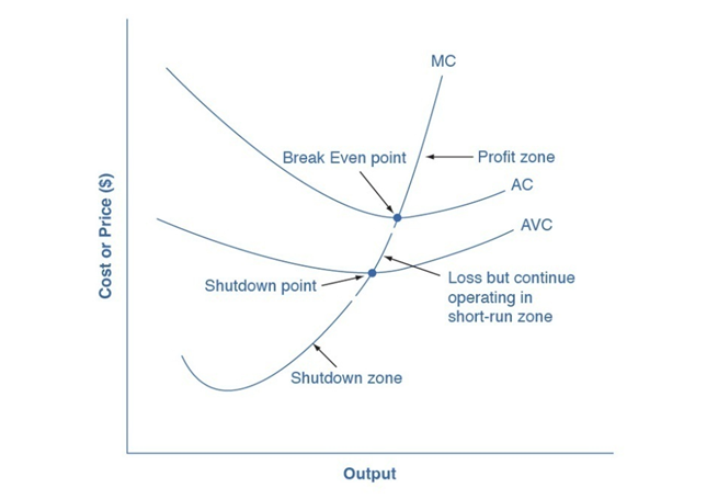
The graph in Figure 10.5 visually represents these scenarios:
- Upper Zone (Profits): When the market price is above the break-even point (where MC intersects AC), the firm makes a profit. The area between the price line and the AC curve up to the quantity produced represents the profit.
- Middle Zone (Operational Losses): Between the break-even point and the shutdown point (where MC intersects AVC), the firm operates at a loss. The area between the AC curve and the price line up to the quantity produced represents the loss. However, since the price is above AVC, the firm covers its variable costs and contributes to fixed costs, minimizing overall losses.
- Lower Zone (Shutdown): At or below the shutdown point, the firm shuts down because it cannot cover its variable costs. The entire fixed cost becomes the loss, as no production occurs.
Summary
In the short run, perfectly competitive firms face three possible outcomes based on the relationship between market price, average cost, and average variable cost:
- Profits: Price > Average Cost (AC)
- Zero Profit: Price = Average Cost (AC)
- Operational Losses: Shutdown Point (AVC) < Price < Average Cost (AC)
- Shutdown: Price ≤ Shutdown Point (AVC)
These outcomes guide firms in deciding whether to continue production or shut down in the short run based on their cost structures and market prices.
Marginal Cost and the Firm’s Supply Curve
In a perfectly competitive market, a firm’s marginal cost (MC) curve is crucial because it directly determines the firm’s supply curve above a certain point. Here’s a detailed explanation:
Definition of Supply Curve:
The supply curve shows the relationship between the price of a good and the quantity a firm is willing to produce and sell at that price.
Decision-Making Process:
Firms decide how much to produce by looking at the market price and comparing it to their costs. The goal is to maximize profits, which occurs where price (P) equals marginal cost (MC).
The Role of Marginal Cost (MC)
- Marginal Cost Curve:
The MC curve represents the cost of producing one additional unit of output. For a perfectly competitive firm, this curve starts from the minimum point on the average variable cost (AVC) curve.
- Profit Maximization:
A firm maximizes profit by producing up to the point where the market price (P) equals the marginal cost (MC). This rule, P = MC, ensures that the firm is not producing units that cost more to make than they earn in revenue.
The Firm’s Supply Curve
- Supply Curve Equals MC Curve:
Since the firm uses the MC curve to decide how much to produce at each price level, the part of the MC curve above the minimum AVC point effectively becomes the firm’s supply curve.
- Minimum AVC as a Threshold:
The supply curve only includes the portion of the MC curve above the minimum AVC because, below this point, the firm would not cover its variable costs and would shut down production.
Numerical Example for a Supply Curve
Consider a firm producing handmade soap in a perfectly competitive market:
- Cost Structure:
- Fixed costs (rent, equipment) are constant regardless of output.
- Variable costs (materials, labor) vary with output.
- Cost Curves:
- Average Variable Cost (AVC): The cost per unit of output, excluding fixed costs.
- Marginal Cost (MC): The additional cost of producing one more unit.
- Production Decisions:
- At a price of $10 per soap, the firm produces where P = MC.
- If the MC at 50 units is $10, the firm will produce 50 units.
- If the market price drops to $8, the firm will produce where MC = $8, say 40 units.
- Shutdown Point:
- If the minimum AVC is $6, and the market price falls below this, the firm stops production because it cannot cover its variable costs.
Graphical Representation
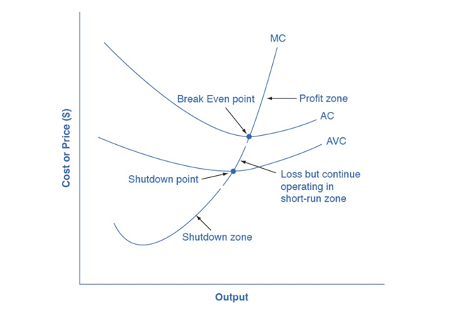
In Figure 10.5 discussed in the previous section, you can visualize the firm’s supply curve:
Zones of MC Curve:
Above Minimum AVC: This segment represents the firm’s supply curve.
Below Minimum AVC: The firm shuts down as it cannot cover variable costs.
Summary
The marginal cost curve, above the minimum average variable cost, serves as the firm’s supply curve in a perfectly competitive market. This relationship holds because profit-maximizing firms produce up to the point where price equals marginal cost, provided the price is above the minimum average variable cost. This ensures firms cover their variable costs and contribute to fixed costs, guiding production decisions effectively.
Entry and Exit of Firms Lead to Zero Profits in the Long Run
In a perfectly competitive market, the forces of entry and exit play a crucial role in driving profits to zero in the long run. Here’s how this process works:
1. Initial Profits Attract New Firms
Profitable Market: When existing firms in a market are making economic profits (where total revenue exceeds total costs), this profitability signals other potential firms to enter the market.
Entry of New Firms: New firms are attracted by the potential to earn profits and start entering the market.
2. Increased Supply Lowers Prices
Increase in Supply: As new firms enter the market, the overall supply of the good increases.
Price Decrease: The increased supply leads to a decrease in the market price of the good. In a perfectly competitive market, firms are price takers, so they must accept the market price.
Reduced Profits: The falling prices reduce the economic profits of all firms in the market.
3. Profits Reach Zero (Normal Profit)
Long-Run Equilibrium: The process of new firms entering the market continues until the economic profits are driven to zero. At this point, firms are making just enough revenue to cover their total costs, including a normal profit (the opportunity cost of the firm’s resources). All firms earn zero economic profits producing an output level where
Zero Economic Profit: When firms make zero economic profit, it means they are covering all their costs (both explicit and implicit) but are not making any excess profit.
4. Losses Lead to Exit
Unprofitable Market: If firms in the market start making losses (where total costs exceed total revenue), some firms will be unable to sustain operations and will exit the market.
Exit of Firms: The exit of firms reduces the total supply of the goods in the market.
5. Decreased Supply Raises Prices
Decrease in Supply: With fewer firms producing the good, the overall supply decreases.
Price Increase: The reduction in supply leads to an increase in the market price of the good.
Reduced Losses: The rising prices reduce the economic losses of the remaining firms.
6. Return to Zero Profit
Long-Run Equilibrium Restored: The process of firms exiting the market continues until the losses are eliminated and firms are again making zero economic profit.
Stable Market: At this point, the market reaches a new long-run equilibrium with zero economic profit for all remaining firms.
Graphical Illustration
The entry and exit of firms in a perfectly competitive market ensure that in the long run, firms will earn zero economic profit. This happens through the following mechanisms:
Entry of new firms reduces profits by increasing supply and lowering prices.
Exit of existing firms reduces losses by decreasing supply and raising prices.
The Long-Run Adjustment and Industry Types
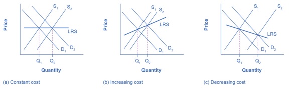
In the long run, the entry and exit of firms in response to profit signals lead to adjustments in the market that can affect the costs of production. These adjustments can categorize industries into three types: constant-cost, increasing-cost, and decreasing-cost industries. Let’s delve into each type and understand the implications with the help of diagrams.
1. Constant-Cost Industry
In a constant-cost industry, as market demand increases, the cost of production for firms remains unchanged.
Adjustment Process:
- Increased Demand: When demand increases, prices initially rise.
- Entry of Firms: New firms enter the market due to the attractive profits.
- Increased Supply: The supply increases until the market returns to the original price but with higher output.
- Result: The long-run supply curve (LRS) is perfectly elastic (horizontal).
Diagram Explanation:
Figure 10.6 (a) shows that as demand increases, the supply also increases proportionally. The equilibrium price stays the same while the quantity increases. The LRS curve is flat, indicating constant costs.
2. Increasing-Cost Industry
Definition: In an increasing-cost industry, as market demand increases, the costs of production for firms increase.
Adjustment Process:
- Increased Demand: Demand increases, causing prices to rise.
- Entry of Firms: New firms enter, but face higher production costs due to limited inputs or rising wages.
- Increased Supply: Supply increases but not enough to offset the increased demand completely.
- Result: The equilibrium price rises, and the LRS curve slopes upward.
Diagram Explanation:
Figure 10.6 (b) depicts that when demand increases, the supply cannot keep up due to higher costs. The equilibrium price increases, and the LRS curve is upward-sloping.
3. Decreasing-Cost Industry
Definition: In a decreasing-cost industry, as market demand increases, the costs of production for firms decrease.
Adjustment Process:
- Increased Demand: Demand increases, raising prices initially.
- Entry of Firms: New firms enter the market, benefiting from lower costs due to factors like technological advancements.
- Increased Supply: Supply increases significantly, leading to lower equilibrium prices.
- Result: The equilibrium price falls, and the LRS curve slopes downward.
Diagram Explanation:
Figure 10.6 (c) illustrates that with increasing demand, supply increases more than demand due to lower costs, reducing the equilibrium price. The LRS curve slopes downward.
Summary of Industry Adjustments
- Constant-Cost Industry: Supply meets increased demand at the same price. The LRS is horizontal.
- Increasing-Cost Industry: Supply increases but not as much as demand, leading to higher prices. The LRS slopes upward.
- Decreasing-Cost Industry: Supply increases more than demand, resulting in lower prices. The LRS slopes downward.
These dynamics ensure that the long-run equilibrium in perfectly competitive markets is reached where firms make zero economic profit, but the paths differ based on how costs adjust with changes in market demand.
Figure 10.6: Adjustment Process
- Figure 10.6 (a): Illustrates a constant-cost industry where increased supply meets increased demand, keeping prices stable.
- Figure 10.6 (b): Illustrates an increasing-cost industry where supply cannot meet demand increases as easily, leading to higher prices.
- Figure 10.6 (c): Illustrates a decreasing-cost industry where supply increases significantly more than demand, causing prices to fall.
Productive Efficiency and Allocative Efficiency in Perfectly Competitive Markets
Perfectly competitive markets are often cited as benchmarks for achieving both productive and allocative efficiency. Here’s how these concepts apply:
Productive Efficiency
Productive efficiency occurs when firms produce goods at the lowest possible cost. This is achieved when the firm operates at the minimum point on its average total cost (ATC) curve.
In Perfect Competition:
- Firms in a perfectly competitive market are driven to minimize costs due to the high level of competition.
- In the long run, only those firms that can produce at the minimum ATC survive, as any firm that cannot, will be driven out of the market.
- This ensures that resources are not wasted and are used the most cost-effectively.
Example:
Imagine a market for wheat. In a perfectly competitive market, all wheat farmers produce wheat at the lowest possible cost due to intense competition. If one farmer can produce wheat more efficiently than others, that farmer will survive and thrive, while less efficient farmers will exit the market. Over time, only the most efficient farmers remain, ensuring that wheat is produced at the lowest cost.
Allocative Efficiency
Allocative efficiency occurs when resources are distributed in a way that maximizes total societal welfare. This happens when the price of a good equals the marginal cost (P = MC) of production.
In Perfect Competition:
- Firms produce up to the point where the price consumers are willing to pay (P) equals the marginal cost (MC) of production.
- This ensures that the value placed on a good by consumers (reflected in the price they are willing to pay) matches the cost of the resources used to produce it.
- No overproduction or underproduction occurs; the quantity supplied equals the quantity demanded at the equilibrium price, maximizing societal welfare.
- The equilibrium point in a perfectly competitive market is where the demand curve (representing consumers’ willingness to pay) intersects the supply curve (representing the marginal cost of production). This intersection (P = MC) ensures allocative efficiency, as the goods produced match consumer preferences and resource costs.
Example:
In the market for milk, allocative efficiency is achieved when the price of milk consumers are willing to pay equals the marginal cost of producing an additional liter of milk. This equilibrium ensures that milk production is perfectly aligned with consumer preferences and societal resources are allocated efficiently.
Summary
Productive Efficiency: Achieved when firms operate at the lowest point on their ATC curve. Perfect competition drives firms to minimize costs, ensuring no resources are wasted.
Allocative Efficiency: Achieved when the price of a good equals the marginal cost of production (P = MC). Perfect competition aligns production with consumer preferences, maximizing societal welfare.
Perfect Competition and Real-World Disparities
In theory, perfectly competitive markets are characterized by several features that ensure both productive and allocative efficiency. When firms in such markets maximize profits by producing the quantity where price (P) equals marginal cost (MC), they ensure that the benefits to consumers from purchasing goods match the costs of producing those goods. This alignment means that resources are allocated efficiently, and no one can be made better off without making someone else worse off.
However, the real-world applicability of perfect competition is limited. Here’s a closer look at why the theoretical model of perfect competition may not hold in practice:
Theoretical Efficiency vs. Real-World Conditions
Income Distribution:
The ability of consumers to pay for goods and services is influenced by income distribution. In reality, income disparities mean that not everyone can afford essential goods, such as cars or healthcare, even if these goods are produced efficiently.
Market Structures:
Most real-world markets are not perfectly competitive. Common market structures like monopoly, oligopoly, and monopolistic competition feature firms that do not produce at the minimum of average cost or set prices equal to marginal cost.
Monopolies can set prices above marginal costs, leading to allocative inefficiency and higher prices for consumers.
Oligopolies may conspire or set prices strategically, also leading to deviations from allocative efficiency.
The monopolistic competition involves differentiated products, where firms have some pricing power and do not produce at the lowest possible cost.
Externalities and Public Goods:
Real-world markets often involve externalities, such as pollution, where the social cost of production is not reflected in market prices.
Public goods like national defense and education are not provided efficiently by private markets because they are non-excludable and non-rivalrous.
Information Asymmetry:
Perfect competition assumes perfect information, where buyers and sellers have complete knowledge about prices and products. In reality, information is often imperfect and unevenly distributed, leading to market failures.
Technological Changes and Innovations:
The model of perfect competition assumes static technology, whereas the real world is dynamic with continuous technological advancements. These changes can disrupt markets and lead to temporary monopolies or oligopolies.
Government Interventions:
Governments intervene in markets through regulations, taxes, and subsidies, which can prevent markets from reaching the ideal of perfect competition.
Diagram Explanation
We will switch to Figure 10.6 for a graphical illustration to elaborate on the disparities.

Constant-Cost Industry: In a constant-cost industry (Figure 10.6a), the long-run supply curve is perfectly elastic. As demand increases, new firms enter the market without increasing production costs, keeping the price constant.
Increasing-Cost Industry: In an increasing-cost industry (Figure 10.6b), the long-run supply curve slopes upward. As new firms enter, the increased demand for inputs raises production costs, leading to higher prices.
Decreasing-Cost Industry: In a decreasing-cost industry (Figure 10.6c), the long-run supply curve slopes downward. As the industry expands, firms benefit from economies of scale or technological improvements, reducing costs and lowering prices.
Summary
While perfect competition provides a useful theoretical benchmark for understanding efficiency, real-world markets often diverge significantly from this model. Factors such as income distribution, market structures, externalities, information asymmetry, technological changes, and government interventions contribute to these differences. Thus, while the concept of perfect competition helps us understand the ideal of productive and allocative efficiency, actual markets frequently fall short of these ideals.
World Around Us: Perfect Competition
Case Study 1: Kodak (Entry, Exit, and Profit Maximization)
Eastman Kodak Company, commonly known as Kodak, was founded by George Eastman in 1888. The company became synonymous with photography, dominating the photographic film market throughout the 20th century. However, Kodak’s journey from a market leader to bankruptcy offers valuable insights into market dynamics, competitive pressures, and strategic mistakes.
Entry into the Market
Kodak entered the photography market in 1888 with its revolutionary “Kodak” camera, which was sold with the slogan, “You press the button, we do the rest.” This innovation made photography accessible to the general public and established Kodak as a pioneer in the industry. The company quickly expanded, offering a wide range of products, including cameras, film, and photographic paper.
Profit Maximization
Kodak enjoyed significant profits throughout much of the 20th century by holding to a business model that focused on selling cameras at relatively low prices while making substantial profits from film sales. This “razor and blades” strategy was highly successful, given the high margins on consumable film products.
Entry of Rivals and Market Changes
Kodak’s dominance began to face challenges with the advent of digital photography in the late 20th century. Companies like Sony, Canon, and Nikon started to innovate in the digital camera space, gradually eroding Kodak’s market share. Despite being a pioneer in digital photography technology (Kodak developed the first digital camera in 1975), the company was slow to shift its business model from film to digital, fearing cannibalization of its profitable film business.
Exit from the Market
By the early 2000s, digital photography had become mainstream, leading to a sharp decline in demand for photographic film. Kodak’s revenues and profits dropped as it struggled to compete with more agile and innovative digital camera manufacturers. In January 2012, Kodak filed for Chapter 11 bankruptcy protection, marking its exit from the core photography market that it had once dominated.
Facts and Figures
- Peak Performance: In 1996, Kodak achieved a peak revenue of $16 billion.
- Digital Transition Delay: Despite inventing the digital camera, Kodak failed to capitalize on digital technology. By the mid-2000s, digital cameras had overtaken film cameras in popularity.
- Market Share Decline: Kodak’s market share in digital cameras fell to single digits by 2010, overshadowed by competitors like Canon and Nikon.
- Bankruptcy: Kodak filed for bankruptcy in January 2012, citing the failure to transition to digital as a primary cause.
Key Concepts: Perfect Competition and Market Dynamics
Entry and Exit: Kodak’s entry into the photography market was marked by innovation and a unique value proposition, which allowed it to dominate. However, the entry of digital competitors and Kodak’s delayed response led to its exit.
Profit Maximization: Kodak’s initial strategy of profit maximization through consumable film sales was highly effective until market conditions changed.
Competitive Pressures: The rise of digital technology and new competitors exemplifies how market dynamics can shift, forcing companies to adapt or exit.
Long-Run Adjustments
Productive Efficiency: In its peak years, Kodak exemplified productive efficiency by leveraging economies of scale in film production. However, its reluctance to shift to digital undermined this efficiency.
Allocative Efficiency: The shift to digital photography improved allocative efficiency in the market, as consumers gained access to better, more convenient technology. Kodak’s failure to align with these preferences led to its decline.
Case Study 2: Blockbuster (Entry, Exit, and Profit Maximization)
Blockbuster LLC, an American-based provider of home movie and video game rental services, was founded in 1985 by David Cook. Blockbuster quickly grew to become a dominant force in the rental industry, with thousands of stores worldwide at its peak.
Entry into the Market
Blockbuster entered the video rental market with a unique approach: a large selection of movies and video games, long store hours, and a standardized, user-friendly layout. This strategy resonated with consumers, leading to rapid expansion and market dominance.
Profit Maximization
Blockbuster maximized profits through a combination of rental fees and late return charges, which became a significant revenue stream. The company also capitalized on the VHS and later DVD rental boom, solidifying its position as a market leader.
Entry of Rivals and Market Changes
The late 1990s and early 2000s saw significant technological advancements and changes in consumer behavior. Netflix, founded in 1997, introduced a new model of DVD rentals by mail, and later, streaming services. Netflix’s subscription-based model eliminated late fees, a key revenue stream for Blockbuster. Despite having the opportunity to purchase Netflix for $50 million in 2000, Blockbuster declined.
Exit from the Market
Blockbuster struggled to adapt to the digital revolution. The company launched its own DVD-by-mail service and attempted to enter the streaming market, but these efforts were too little, too late. By 2010, Blockbuster filed for bankruptcy, and by 2014, most of its stores were closed, marking its exit from the market.
Facts and Figures
- Peak Performance: In 2004, Blockbuster had over 9,000 stores worldwide.
- Missed Opportunity: Blockbuster’s failure to purchase Netflix in 2000 for $50 million.
- Bankruptcy: Filed for Chapter 11 bankruptcy in September 2010.
- Decline: By 2014, only a few stores remained open, mostly franchisee-owned.
Key Concepts: Perfect Competition and Market Dynamics
Entry and Exit: Blockbuster entered the market with a strong value proposition but failed to adapt to new competition and technological changes, leading to its exit.
Profit Maximization: Blockbuster initially maximized profits through rental and late fees but could not sustain this model in the face of new competition.
Long-Run Adjustments
Productive Efficiency: Blockbuster’s large-scale operations and standardized stores exemplified productive efficiency initially. However, the inability to adapt to digital transformation undermined this efficiency.
Allocative Efficiency: Netflix and other streaming services improved allocative efficiency by offering consumers greater convenience and a broader selection of content.
Case Study 3: Nokia (Entry, Exit, and Profit Maximization)
Nokia Corporation, originally a paper mill, evolved into a telecommunications giant, becoming the world leader in mobile phones in the late 1990s and early 2000s. Founded in 1865, Nokia’s entry into telecommunications in the 1980s marked its transformation.
Entry into the Market
Nokia entered the telecommunications market by producing mobile phones and network infrastructure. The company’s focus on innovation, quality, and branding led to rapid market penetration and dominance.
Profit Maximization
Nokia maximized profits through economies of scale, extensive distribution networks, and a strong brand presence. The company continually innovated with new mobile phone models, catering to various market segments and maintaining a competitive edge.
Entry of Rivals and Market Changes
The smartphone revolution, led by Apple’s iPhone in 2007 and Google’s Android platform, drastically changed the mobile phone landscape. Nokia’s reliance on its Symbian operating system, which could not compete with the user experience offered by iOS and Android, put the company at a disadvantage. Despite attempts to innovate, Nokia’s market share eroded rapidly.
Exit from the Market
In 2011, Nokia partnered with Microsoft to adopt the Windows Phone operating system, hoping to regain its competitive edge. However, the partnership failed to produce significant market share gains. By 2013, Nokia sold its mobile phone business to Microsoft, effectively exiting the market it once led.
Facts and Figures
- Peak Performance: In 2007, Nokia held a 49.4% market share in mobile phones.
- Decline: By 2013, Nokia’s market share had fallen to single digits.
- Acquisition: In 2013, Nokia sold its mobile phone division to Microsoft for $7.2 billion.
Key Concepts: Perfect Competition and Market Dynamics
- Entry and Exit: Nokia’s entry into telecommunications was marked by innovation and strategic positioning. However, the failure to adapt to the smartphone revolution led to its exit.
- Profit Maximization: Nokia initially maximized profits through innovation and market dominance but could not sustain this as the market evolved.
Long-Run Adjustments
- Productive Efficiency: Nokia’s production processes and global supply chain exemplified productive efficiency. However, the inability to compete in the smartphone market undermined this efficiency.
- Allocative Efficiency: The rise of smartphones improved allocative efficiency by offering consumers advanced technology and better user experiences, which Nokia failed to provide.
Razor and Blades Strategy
The “razor and blades” strategy is a business model where a company sells a primary product (the “razor”) at a low price, often at a loss, to generate sales of complementary consumable products (the “blades”) at a higher margin.
Example: A classic example is Gillette, which sells its razors at a low price or gives them away for free to boost sales of razor blades, which are more profitable.
Application:
- Video Game Consoles: Companies like Sony and Microsoft sell gaming consoles at or below cost to encourage the purchase of profitable video games and accessories.
- Printers and Ink Cartridges: Printer manufacturers sell printers cheaply but charge high prices for ink cartridges.
Benefits:
- Builds a customer base quickly.
- Generates steady revenue from the consumables.
- Encourages brand loyalty as customers repeatedly buy the consumables.
Challenges:
- Initial losses on the primary product.
- Requires effective marketing to ensure high sales of the consumables.
- Potential competition on the consumable products can affect profitability.
The strategy relies on the idea that ongoing sales of the consumables will compensate for the low-margin or loss-leading primary product, leading to overall profitability.
Quasi-Perfectly Competitive Market
A quasi-perfectly competitive market is a market structure that closely resembles perfect competition but has some deviations from it.
Characteristics:
- Many Sellers and Buyers:
There are numerous sellers and buyers, but not as many as in a perfectly competitive market.
- Product Differentiation:
Products are similar but not identical. Each firm offers a slightly different version.
- Free Entry and Exit:
Firms can enter or leave the market without significant barriers.
- Price Maker:
Firms have some control over their prices due to product differentiation.
- Imperfect Information:
Buyers and sellers do not have complete information about prices and products.
Example: Observe a local market for handmade crafts. There are many sellers, but each offers unique items. Buyers can choose from different products, but they have some flexibility in prices.
Key Point: A quasi-perfectly competitive market is close to perfect competition but allows for some product differences and limited pricing power.
Impact of Globalization on the Principles of Perfect Competition
Globalization refers to the increasing interconnectedness and interdependence of the world’s markets and businesses. It has significant effects on the principles of perfect competition, which include numerous small firms, homogeneous products, perfect information, and free entry and exit from the market. Here are the key impacts of globalization:
1. Increased Market Size
Expansion of Markets: Globalization expands the market size beyond local or national borders. Firms can access a larger pool of consumers, potentially increasing demand for their products.
Scale Economies: Larger markets allow firms to achieve economies of scale, reducing average costs and potentially increasing competition.
2. Enhanced Competition
Entry of Foreign Firms: Globalization facilitates the entry of foreign firms into domestic markets, increasing the number of competitors.
Competitive Pressure: Domestic firms face greater competitive pressure to improve efficiency, lower costs, and innovate to maintain market share.
3. Product Homogeneity
Standardization: Globalization can lead to the standardization of products and services, making them more homogeneous across markets. This aligns with the perfect competition assumption of identical products.
Diverse Preferences: However, globalization also brings diverse consumer preferences, which can lead to product differentiation, deviating from perfect competition.
4. Information Flow
Improved Information Access: Globalization enhances the flow of information through the Internet and other communication technologies, helping consumers and firms make informed decisions.
Information Asymmetry: Despite improvements, information asymmetry may still exist due to language barriers, cultural differences, and varying regulations.
5. Free Entry and Exit
Reduced Barriers: Globalization reduces barriers to entry and exit by harmonizing regulations, reducing tariffs, and encouraging trade agreements.
Market Dynamics: The ease of entry and exit fosters a dynamic market environment where inefficient firms are quickly replaced by more competitive ones.
6. Cost Structures
Labor Costs: Firms can optimize labor costs by outsourcing production to countries with lower wages, affecting the cost structures and competitive dynamics.
Input Availability: Access to global supply chains can reduce input costs and enhance efficiency.
7. Innovation and Technology
Technology Transfer: Globalization facilitates the transfer of technology and innovation across borders, enhancing productivity and competitiveness.
R&D Investments: Increased competition encourages firms to invest in research and development to differentiate their products and reduce costs.
8. Regulatory Environment
Harmonized Standards: Globalization often leads to harmonized standards and regulations, simplifying compliance for firms operating in multiple countries
Regulatory Challenges: Firms must navigate different regulatory environments, which can be complex and costly.
Summary
Globalization profoundly impacts the principles of perfect competition by expanding markets, enhancing competition, improving information flow, and reducing barriers to entry and exit. While it aligns with some aspects of perfect competition, such as increasing the number of firms and standardizing products, it also introduces complexities like information asymmetry and diverse consumer preferences. Overall, globalization creates a more competitive and dynamic market environment, pushing firms toward greater efficiency and innovation.
Role of Consumer Surplus in Perfectly Competitive Markets
Consumer surplus is a critical concept in the analysis of perfectly competitive markets. It measures the difference between what consumers are willing to pay for a good or service and what they pay. This surplus provides insights into the benefits consumers receive from market transactions and plays several key roles in the analysis of perfectly competitive markets:
1. Indicator of Welfare
Consumer Benefit: Consumer surplus reflects the overall benefit that consumers receive from purchasing goods and services at market prices lower than their maximum willingness to pay. In a perfectly competitive market, where prices are determined by the intersection of supply and demand, consumer surplus indicates the welfare gains to consumers.
Market Efficiency: High consumer surplus in a perfectly competitive market suggests that the market is efficient and consumers are deriving maximum benefit from transactions.
2. Measurement of Market Efficiency
Allocative Efficiency: In perfectly competitive markets, allocative efficiency is achieved when the price of a good equals the marginal cost of production (P = MC). At this point, the consumer surplus is maximized because consumers are paying a price equal to the cost of producing the last unit they consume.
Productive Efficiency: Perfect competition also ensures productive efficiency, where goods are produced at the lowest possible cost. This efficiency translates into lower prices for consumers, thereby increasing consumer surplus.
3. Impact of Market Changes
Price Changes: Consumer surplus is sensitive to changes in market prices. In a perfectly competitive market, if supply increases (shifting the supply curve right), prices fall, and consumer surplus increases. Conversely, if supply decreases, prices rise, and consumer surplus decreases.
Entry and Exit of Firms: The entry of new firms into a perfectly competitive market increases supply, reduces prices, and increases consumer surplus. The exit of firms reduces supply, increases prices, and reduces consumer surplus.
4. Economic Policy Analysis
Policy Evaluation: Consumer surplus is often used to evaluate the impact of economic policies, such as taxes, subsidies, and price controls. For example, a subsidy that lowers the price of a good increases consumer surplus, indicating a benefit to consumers.
Welfare Comparisons: By comparing consumer surplus before and after a policy intervention, economists can assess the welfare implications of different policy choices.
5. Dynamic Efficiency and Innovation
Innovation Benefits: In a perfectly competitive market, firms are incentivized to innovate to reduce costs and differentiate their products. The successful innovations, that lower production costs lead to lower prices and higher consumer surplus.
Long-Term Benefits: Sustained innovation and cost reductions over time can lead to significant increases in consumer surplus, reflecting long-term benefits to consumers from technological advancements and improved market efficiency.
Summary
Consumer surplus is a vital measure of consumer welfare and market efficiency in perfectly competitive markets. It provides insights into the benefits consumers receive from market transactions, the efficiency of resource allocation, and the impact of market changes and policy interventions. By maximizing consumer surplus, perfectly competitive markets ensure that consumers derive the greatest possible benefit from economic activities, contributing to overall economic well-being.
Lessons for Policymakers from the Model of Perfect Competition
The model of perfect competition offers several valuable lessons for policymakers when designing economic regulations. Here are the key suggestions:
1. Promote Competition
Avoid Monopolies and Oligopolies: Ensure market structures remain competitive to prevent monopolies and oligopolies that can lead to higher prices, reduced output, and decreased consumer welfare.
Anti-Trust Laws: Implement and enforce antitrust laws to break up monopolies and prevent anti-competitive practices such as collusion and price-fixing.
2. Encourage Entry and Exit
Lower Barriers to Entry: Reduce regulations and costs that restrict new firms from entering the market. This encourages innovation, diversity, and competitive pressures.
Support for Exit: Ensure that the process of exiting the market is not overly burdensome for firms, allowing resources to be reallocated efficiently.
3. Ensure Transparent and Informative Markets
Access to Information: Promote transparency and provide consumers and firms with access to accurate, timely information. This helps in making informed choices and fosters competition.
Reduce Asymmetry: Work to eliminate information asymmetry between buyers and sellers to ensure a level playing field.
4. Regulate Fairly to Maintain Efficiency
Balancing Regulation: While regulation is necessary, it should be designed to maintain market efficiency without oppressing innovation or competition. Avoid overly restrictive regulations that can create monopolistic conditions.
Focus on Market Failures: Target regulations to address market failures such as externalities, public goods, and information asymmetries, without distorting competition.
5. Promote Productive and Allocative Efficiency
Encourage Innovation: Support research and development and provide incentives for technological advancements, which can reduce costs and improve product quality, enhancing consumer welfare.
Align Prices with Costs: Ensure that prices reflect the true cost of production, including external costs, to promote allocative efficiency where P = MC.
6. Consider Long-Term Market Dynamics
Support Dynamic Competition: Promote an environment where firms are encouraged to innovate and improve efficiency over time, maintaining long-term competitive pressure.
Monitor and Adjust Policies: Continuously monitor market conditions and be prepared to adjust regulations to address emerging challenges and maintain market competitiveness.
7. Address Market Inequities
Consider Equity in Policy Design: Design policies that consider income distribution and social equity, ensuring that the benefits of competition and market efficiency are widely shared.
Support Vulnerable Groups: Implement safety nets and support mechanisms for vulnerable populations who may be adversely affected by market dynamics.
8. Facilitate Market Integration and Global Competition
Promote Free Trade: Encourage policies that enhance global trade and competition, enabling local firms to access international markets and benefit from global efficiencies.
Harmonize Standards: Work towards harmonizing regulations and standards with international norms to reduce trade barriers and enhance market integration.
Summary
By integrating these lessons, policymakers can create a regulatory environment in which rising competition enhances market efficiency and ensures consumer welfare while addressing market failures and promoting equitable growth. The goal is to manage the strengths of perfect competition to design policies that support a dynamic, innovative, and fair economic system.
Perfect Competition through the Lens of Behavioral Economics
Perfect competition assumes that consumers and producers act rationally, seeking to maximize utility and profit, respectively. All firms in a perfectly competitive market are price takers, with identical products and no barriers to entry or exit. However, behavioral economics suggests that real-world decisions often deviate from these assumptions due to cognitive biases, emotions, and other psychological factors.
Scenario: Farmers in a Wheat Market
Imagine a large group of farmers selling wheat in a perfectly competitive market. According to traditional economic theory, each farmer should produce at a level where marginal cost equals market price, ensuring maximum profit.
Cognitive Biases
- Loss Aversion: Farmers might be reluctant to lower their output or exit the market even when prices drop below production costs. They fear losing their farms or income, which might lead them to continue producing at a loss, rather than reallocating resources to more profitable ventures.
- Overconfidence Bias: Some farmers might overestimate their ability to withstand market downturns, invest in expensive machinery or expand production when prices are temporarily high. This can lead to financial strain when prices normalize.
Prospect Theory
- Reference Points: Farmers might consider past high prices as reference points. When current prices are lower, they perceive these as losses, leading them to take unnecessary risks, like taking loans to maintain production levels.
- Framing Effect: How market conditions are presented influences decisions. If a price drop is framed as a temporary setback, farmers might continue producing, believing prices will recover, even when long-term trends suggest otherwise.
World Around Us: Behavioral Economics
Case Study: Dairy Farmers in New Zealand
New Zealand’s dairy industry is one of the most competitive and globally integrated sectors. The market operates under conditions close to perfect competition, with numerous farmers producing homogenous products (milk) and facing international market prices. However, behavioral factors often influence decision-making, leading to outcomes that deviate from standard economic predictions.
Key Findings of the Study
Production Despite Falling Milk Prices
- Even as global milk prices declined, many farmers continued production, despite incurring losses.
- Farmers were reluctant to scale back production, believing that cutting back would lead to greater losses in the long run.
Cognitive Biases at Play
- Loss Aversion:
- Farmers viewed reducing production as a loss, even if it might have been a rational decision.
- They preferred to maintain production levels, even at a loss, to avoid admitting or experiencing a perceived “defeat.”
- Overconfidence:
- Over 30% of farmers expected milk prices to rebound within a year.
- This overconfidence in a quick recovery led them to overestimate the future profitability of their production decisions.
- Sunk Cost Fallacy:
- Many farmers had already invested heavily in infrastructure, equipment, and feed.
- They considered these past investments when deciding to continue production, even though these costs were non-recoverable.
Behavioral Dynamics and Emotional Responses
Optimism and Risk-Taking
- Farmers demonstrated optimism about market recovery, which contributed to their reluctance to adjust production.
- They took on additional debt, believing they could cover it once prices improved.
Emotional Attachment to Farming
- For many farmers, dairy production was more than a business—it was a livelihood tied to family traditions.
- This emotional attachment amplified their resistance to change, making them prioritize continuity over financial prudence.
Market Implications
Overproduction and Price Declines
- Farmers, influenced by behavioral factors, produced more milk than the market could absorb.
- This oversupply further depressed global milk prices, creating a vicious cycle.
Financial Stress
- Continuing production at a loss increased debt burdens.
- Many small-scale farmers struggled to remain solvent, with some leaving the market entirely after extended losses.
Lessons for Policy and Market Behavior
- Behavioral Interventions:
- Providing education on market trends and psychological training could help farmers make more rational decisions.
- Behavioral nudges, such as offering financial incentives for scaling back production, might align individual decisions with market realities.
- Market Stabilization Mechanisms:
- Governments or industry bodies could introduce temporary production quotas to prevent overproduction during periods of low prices.
- Psychological Awareness in Policy Design:
- Policies should consider the impact of cognitive biases like loss aversion and overconfidence.
- Emotional and psychological factors should be addressed alongside economic solutions.
Impact and Analysis
This case study highlights the role of behavioral economics in shaping decisions, even in markets with conditions close to perfect competition. Key observations include:
- Behavioral Factors:
- Loss aversion and overconfidence led farmers to persist in loss-making production.
- Emotional and psychological considerations often override rational calculations.
- Economic Consequences:
- Suboptimal decisions by individual farmers resulted in collective oversupply, driving prices further down.
- This underscores the need for integrating behavioral insights into agricultural policy and market management strategies.
By understanding the behavioral dynamics in such scenarios, policymakers and industry leaders can develop solutions that reduce the impact of cognitive biases, fostering both individual and market-level sustainability.
References
- Kahneman, D. (2011). Thinking, Fast and Slow.
- Tversky, A., & Kahneman, D. (1979). Prospect Theory: An Analysis of Decision under Risk.
- Thaler, R. H., & Sunstein, C. R. (2008). Nudge: Improving Decisions About Health, Wealth, and Happiness.
- New Zealand Dairy Farmers Study (2019).
Research Suggestions in Behavioral Economics
1. Market Exit Decisions
- Investigate how loss aversion and emotional attachment to businesses affect the decision to exit a market, particularly in agriculture or small businesses.
2. Price Perception and Decision-Making
- Study how the framing of market price information (e.g., as a loss or gain) influences production decisions in competitive markets.
3. Behavioral Responses to Market Volatility
- Explore how overconfidence bias affects investment and production decisions in volatile markets like agriculture or commodities.
4. Impact of Behavioral Nudges
- Examine how behavioral nudges (like financial planning tools) could help farmers or small producers make more rational decisions in the face of fluctuating prices.
5. Behavioral Economics in Agricultural Policy
- Research how government policies can incorporate behavioral insights to encourage more rational production decisions and reduce market inefficiencies.
This approach to understanding perfect competition through the lens of behavioral economics reveals the complexity of real-world decision-making and the importance of considering psychological factors in economic models.
Critical Thinking
- How does the concept of perfect competition apply to real-world markets?
- What are the main characteristics of a perfectly competitive market?
- Why is it difficult to find perfectly competitive markets in reality?
- How does a firm in a perfectly competitive market determine its profit-maximizing output level?
- What role does the assumption of “many buyers and sellers” play in ensuring perfect competition?
- How do perfect knowledge and information affect the efficiency of perfectly competitive markets?
- Explain how the entry and exit of firms ensure zero economic profit in the long run.
- How do differences in cost structures among firms affect competition in a perfectly competitive market?
- What is the significance of the marginal cost (MC) curve in determining a firm’s supply curve in perfect competition?
- How does perfect competition ensure allocative efficiency?
- Why might a perfectly competitive market fail to achieve productive efficiency in the short run?
- How do external factors like government regulation or technological changes impact perfect competition?
- Discuss the role of sunk costs in the decision-making process of firms in perfect competition.
- What are the implications of a perfectly elastic supply curve in a constant-cost industry?
- How does a decreasing-cost industry differ from an increasing-cost industry in terms of long-run supply curve behavior?
- What are the potential effects of entry and exit barriers on a perfectly competitive market?
- How do perfectly competitive markets respond to changes in consumer preferences?
- How does the assumption of identical products contribute to the model of perfect competition?
- What are the welfare implications of perfect competition for consumers and producers?
- How does perfect competition address issues of equity and income distribution?
- Discuss the potential limitations of using perfect competition as a benchmark for real-world markets.
- How does the entry of new firms into a perfectly competitive market affect prices and output in the short run and long run?
- Explain the concept of the shutdown point for a firm in a perfectly competitive market.
- How does technological advancement influence the dynamics of a perfectly competitive industry?
- Discuss the impact of globalization on the principles of perfect competition.
- What role does consumer surplus play in the analysis of perfectly competitive markets?
- How does perfect competition ensure that resources are allocated to their most valued uses?
- What lessons can policymakers learn from the model of perfect competition when designing economic regulations?
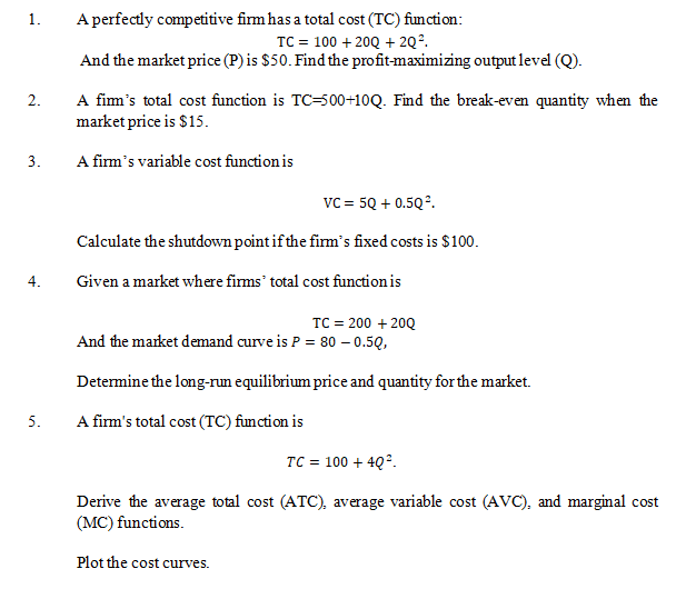
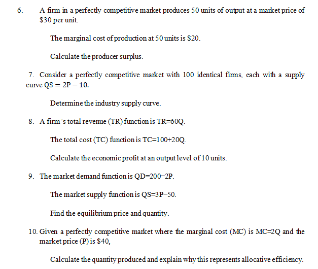
Numerical Problems: Perfect Competition



3 Comments