Now we will explore the fascinating world of elasticity. This concept is crucial for understanding how changes in prices and other factors affect demand and supply. For instance, if the price of a popular smartphone increases, knowing its price elasticity helps predict how much the demand will drop. A company can set prices to maximize revenue. Governments will exercise elasticity to predict the effects of taxes and subsidies. Hence elasticity has different types and impacts so we will explore them in detail.

Price Elasticity of Demand and Supply

Price Elasticity of Demand (PED): Measures how much the quantity demanded of a good responds to a change in the price of that good.

Or it is the ratio of the percentage change in quantity demanded to the percentage change in price during the given period of time.

Price Elasticity of Supply (PES): Measures how much the quantity supplied of a good responds to a change in the price of that good.

Or it is the ratio of percentage change in quantity supplied to the percentage change in price during the given period of time.

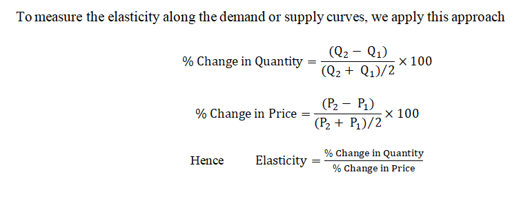
Price Elasticity of Demand (PED):

Price Elasticity of Demand (PED) measures the responsiveness of the quantity demanded of a good to a change in its price. In simpler terms, it indicates how much the demand for a product changes when its price changes.

Interpretation of PED Values

1. Elastic Demand: When the % change in quantity demanded is greater than the % change in price. (PED > 1)
2. Unitary Demand: When the % change in quantity demanded is equal to the % change in price. (PED = 1)
3. Inelastic Demand: When the % change in quantity demanded is less than the % change in price. (PED < 1)

Elaborate on these three scenarios:

Elastic Demand (PED > 1)

If the percentage change in quantity demanded is greater than the percentage change in price, the demand is considered elastic.

Or if % change in quantity > % change in price (PED > 1) Then the demand is elastic.

Example: If a 10% decrease in the price of a luxury car results in a 20% increase in the quantity demanded, the PED is 2 (20%/10%).

Unitary Demand (PED = 1)

If the percentage change in quantity demanded is equal to the percentage change in price, the demand is considered unitary.

Or if % change in quantity = % change in price (PED = 1) Then the demand is unitary.

Example: If a 10% decrease in the price of a smartphone results in a 10% increase in the quantity demanded, the PED is 1 (10%/10%).

Inelastic Demand (PED < 1)

If the percentage change in quantity demanded is less than the percentage change in price, the demand is considered inelastic.

Or if % change in quantity < % change in price (PED < 1) Then the demand is inelastic.

Example: If a 10% decrease in the price of gasoline results in only a 5% increase in the quantity demanded, the PED is 0.5 (5%/10%).

Measuring Price Elasticity of Demand

Let’s revert to our reference book with the following example:

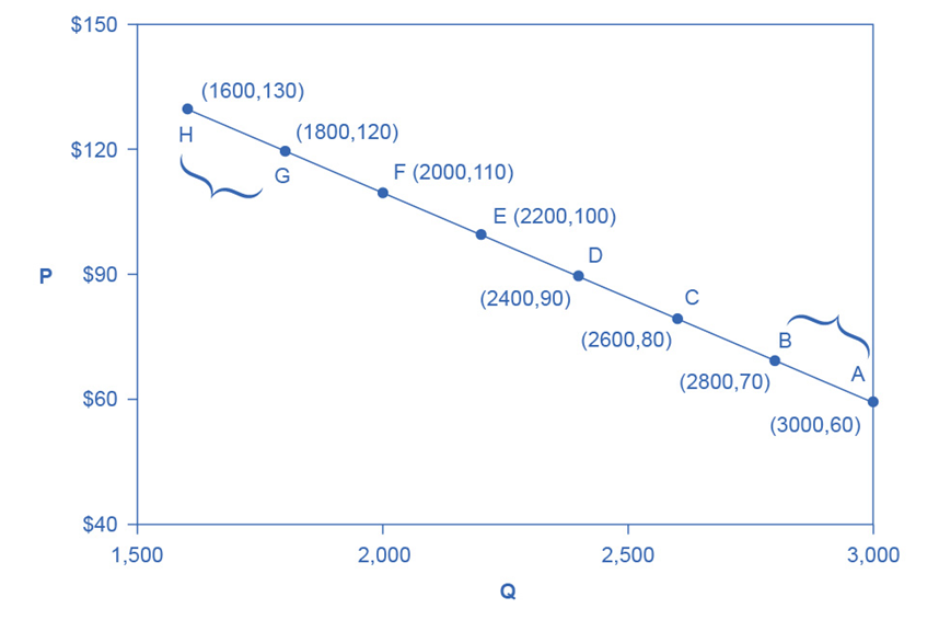
• Point H: Price = $130, Quantity = 1600
• Point G: Price = $120, Quantity = 1800
• Point B: Price = $70, Quantity = 2800
• Point A: Price = $60, Quantity = 3000

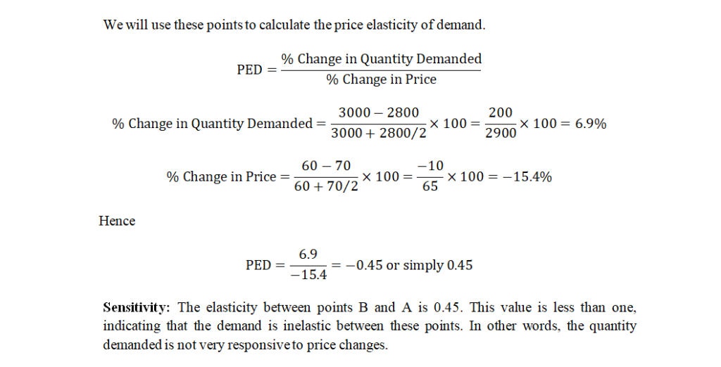
• If the price changes by 1%, the quantity demanded will change by 0.45%.
• A 10% increase in price will lead to only a 4.5% decrease in quantity demanded.
• A 10% decrease in price will lead to only a 4.5% increase in quantity demanded.

Although price elasticities of demand are negative because price and quantity move in opposite directions, we usually interpret them as positive values for simplicity.

Factors Influencing PED

1. Availability of Substitutes: Goods with many substitutes tend to have higher elasticity.
2. Necessity vs. Luxury: Necessities tend to have inelastic demand, while luxuries are more elastic.
3. Proportion of Income: Goods that take up a larger proportion of income tend to have more elastic demand.
4. Time Period: Demand is usually more elastic over the long run than the short run.

World around Us: Price Elasticity of Demand

Case Study 1: Airline Tickets in Southeast Asia

• Airlines often engage in competitive pricing, especially during off-peak seasons.
• In 2019, a major airline reduced ticket prices by 15% to increase passenger numbers.
• The reduction led to a 30% increase in the number of tickets sold.
• PED = 2 (30% / 15%), indicating elastic demand. The demand for airline tickets is highly responsive to price changes due to the availability of substitutes (other airlines and travel modes).

Case Study 2: Cigarettes in Pakistan

• The government increased taxes on cigarettes to reduce smoking rates.
• In 2020, the price of a pack of cigarettes increased by 20%.
• The quantity demanded decreased by only 5%.
• PED = 0.25 (5% / 20%), indicating inelastic demand. Cigarettes are a necessity for smokers, leading to less responsiveness to price changes.

Case Study 3: Smartphone Market in India

• A leading smartphone brand launched a new model with a 10% price cut during a festival season.
• In 2021, the price of the new smartphone model was reduced by 10%.
• The quantity demanded increased by 15%.
• PED = 1.5 (15% / 10%), indicating elastic demand. Consumers in India are highly responsive to price changes in the competitive smartphone market with many alternatives.

In summary, the price elasticity of demand measures how sensitive the quantity demanded of a good is to a change in its price. In our example, the demand between points B and A is inelastic, meaning changes in price lead to smaller percentage changes in quantity demanded.

---

Price Elasticity of Supply (PES)

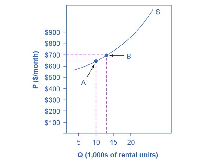
Price Elasticity of Supply (PES) measures the responsiveness of the quantity supplied of a good to a change in its price. It indicates how much the supply of a product changes when its price changes.

Elaboration on these three scenarios:

Elastic Supply (PES > 1)

If the percentage change in quantity supplied is greater than the percentage change in price, the supply is considered elastic.

Or if % change in quantity > % change in price (PES > 1) Then the supply is elastic.

Example: If a 10% increase in the price of strawberries results in a 20% increase in the quantity supplied, the PES is 2 (20%/10%).

Unitary Supply (PES = 1)

If the percentage change in quantity supplied is equal to the percentage change in price, the supply is considered unitary.

Or if % change in quantity = % change in price (PES = 1) Then the supply is unitary.

Example: If a 10% increase in the price of handmade jewelry results in a 10% increase in quantity supplied, the PES is 1 (10%/10%).

Inelastic Supply (PES < 1)

If the percentage change in quantity supplied is less than the percentage change in price, the supply is considered inelastic.

Or if % change in quantity < % change in price (PES < 1) Then the supply is inelastic.

Example: If a 10% increase in the price of apartments results in only a 5% increase in the quantity supplied, the PES is 0.5 (5%/10%).

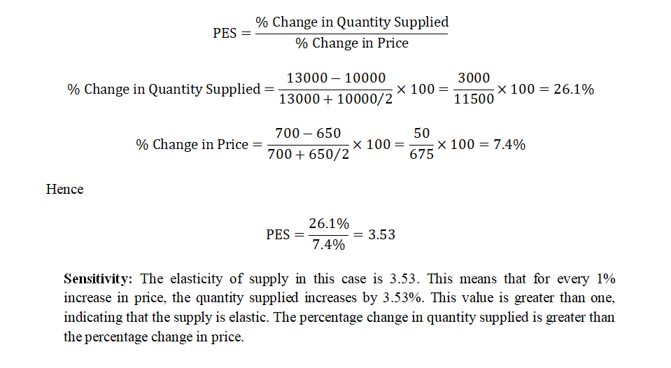
Measuring Price Elasticity of Supply

Let’s revert to our reference book with following example:

Factors Influencing PES

1. Time Period: Supply is generally more elastic in the long run than in the short run because producers have more time to adjust their production levels.
2. Availability of Resources: If resources required to produce a good are readily available, supply tends to be more elastic.
3. Flexibility of Production: If production processes can be easily modified, supply tends to be more elastic.
4. Spare Capacity: If a firm has spare production capacity, it can increase output without a rise in costs, leading to more elastic supply.

World around Us: Price Elasticity of Supply

Case Study 1: Agricultural Produce in India

• The supply of agricultural products can vary greatly due to factors such as weather conditions.
• In 2016, the price of tomatoes increased by 50% due to a poor harvest season.
• Despite the price increase, the quantity supplied only increased by 20% because it takes time to grow more tomatoes.
• PES = 0.4 (20% / 50%), indicating inelastic supply. The supply of agricultural products is often inelastic in the short term due to the time required for production.

Case Study 2: Oil Production in Saudi Arabia

• Oil production involves significant investment and infrastructure, making it less responsive to price changes.
• In 2018, global oil prices increased by 30%.
• Saudi Arabia’s oil production increased by 10%.
• PES = 0.33 (10% / 30%), indicating inelastic supply. Oil production is less responsive to short-term price changes due to the complexity and cost of adjusting production levels.

Case Study 3: Handicrafts in Bangladesh

• Handicrafts are often produced by small-scale artisans who can quickly respond to price changes.
• In 2021, the price of traditional Bangladeshi hand-woven textiles increased by 15% due to a surge in demand.
• The quantity supplied increased by 25% as artisans increased production.
• PES = 1.67 (25% / 15%), indicating elastic supply. Handicraft production is more elastic due to the flexibility and small-scale nature of the industry.

---

Impact of Technology on Elasticity

Technology has a significant impact on both the price elasticity of demand (PED) and the price elasticity of supply (PES). Technological advancements can make products more affordable, production processes more efficient, and markets more dynamic

Impact on Price Elasticity of Demand (PED)

Product Innovation and Variety: The smartphone market.

Technological advancements have led to a wide variety of smartphones with different features and price points. This variety increases consumer choices, making demand more elastic as consumers can easily switch to different models or brands if prices rise.

Substitute Goods: Streaming services.

The rise of technology has introduced numerous streaming services (e.g., Netflix, Amazon Prime, Hulu). If one service raises its prices, consumers can easily switch to another, making the demand for any single service more elastic.

Price Comparison and Information Availability: E-commerce platforms

Online shopping platforms like Amazon and Alibaba provide consumers with easy access to price comparisons and reviews. This transparency increases demand elasticity, as consumers can quickly find and switch to cheaper alternatives.

Technology Impact on Price Elasticity of Supply (PES)

Production Efficiency: Automotive manufacturing.

Automation and advanced manufacturing technologies have made it easier for car manufacturers to scale production up or down quickly in response to price changes. This increased flexibility leads to more elastic supply.

Supply Chain Management: Fast fashion.

Different renowned clothing brands worldwide use sophisticated supply chain technologies to respond rapidly to fashion trends. This agility makes their supply more elastic as they can quickly increase production to meet demand.

Digital Platforms: Ride-sharing services.

Platforms like Uber and Lyft use technology to match supply (drivers) with demand (riders) in real-time. This dynamic adjustment capability results in a highly elastic supply of ride-sharing services.

World around Us: Impact of Technology on Elasticity

Case Study 1: E-Commerce in China

• The rapid growth of e-commerce platforms like Alibaba and JD.com.
• During the annual Singles’ Day shopping festival in 2020, Alibaba sales surpassed $74 billion.
• The availability of various products and easy price comparisons made consumer demand highly elastic.
• Advanced logistics and supply chain technologies allowed sellers to quickly restock and meet the surge in demand, indicating an elastic supply.

Case Study 2: Electric Vehicles (EVs) in Europe

• The increasing adoption of electric vehicles due to technological advancements and environmental concerns.
• In 2020, Europe saw a 137% increase in EV sales compared to the previous year.
• The introduction of more affordable EV models and government incentives made demand more elastic.
• Advances in battery technology and production efficiency enabled manufacturers to scale production, resulting in more elastic supply.

Case Study 3: Agriculture Technology in India

• Adoption of precision agriculture technologies like drones and sensors.
• The Indian government’s push for digital agriculture in 2021 aimed to double farmers’ income.
• Improved crop quality and yield diversification made agricultural products more competitive, affecting demand elasticity.
• Precision agriculture allowed farmers to optimize production based on real-time data, making supply more responsive to price changes and thus more elastic.

Practical Examples of Technological Impact on Elasticity

• If technology improves production efficiency (e.g., automation in factories), then the supply becomes more elastic because producers can quickly adjust output levels.
• If technology enhances consumer access to information (e.g., price comparison websites), then the demand becomes more elastic as consumers can easily switch to alternatives.
• If technology reduces production costs (e.g., renewable energy technologies), then the supply becomes more elastic as firms can produce more at lower costs.

Is the elasticity the slope?

We can compare and find the differences between these two concepts as followings:

Slope	Elasticity
The slope measures the rate at which one variable changes in relation to another variable.	Elasticity measures the percentage change in one variable resulting from a 1% change in another variable.
It is calculated as the change in the y-variable divided by the change in the x-variable (Δy/Δx).	Specifically, price elasticity of supply or demand calculates the percentage change in quantity supplied or demanded divided by the percentage change in price.
In the context of supply and demand curves, the slope shows how much the quantity supplied or demanded changes when the price changes by one unit.	It measures the sensitive of the quantity supplied or demanded is to a change in price, regardless of the units of measurement.
Slope is expressed in the units of the variables (e.g., dollars per unit for price per quantity).	Elasticity is a ratio of percentages and is unit less.
Slope gives the rate of change between two variables.	Elasticity tells us the relative responsiveness of quantity to price changes.

---

Determinants of Elasticity

Price elasticity of demand and supply is influenced by several key factors. Understanding these determinants helps us predict how changes in price will affect the quantity demanded or supplied. Here, we will explore the main determinants and provide real-world case studies to illustrate these concepts.

1. Availability of substitutes
2. Necessity vs. luxury
3. Proportion of income spent on the good
4. Time Horizons
5. Definition of the Market

Availability of Substitutes

The more substitutes available for a product, the more elastic the demand for it tends to be. Consumers can easily switch to a substitute if the price of the original product rises.

Case Study: Soft Drink Market

• The market for soft drinks is highly competitive with many available substitutes such as juices, bottled water, and energy drinks.
• When the price of a specific brand of soft drink increases, consumers can easily switch to another brand or a different beverage.
• Example: In 2018, Coca-Cola faced increased competition from healthier beverage options. According to Beverage Digest, the U.S. soda market volume fell by 1.7%, and Coca-Cola’s sales decreased by 2% when the company increased prices by 5%. This drop in sales occurred as consumers shifted to alternatives like flavored water and organic juices, illustrating high elasticity.

Necessity vs. Luxury

Necessities tend to have inelastic demand because consumers need them regardless of price changes. Luxuries, on the other hand, have more elastic demand because they are non-essential and often have substitutes.

Case Study: Pharmaceutical Drugs

• Life-saving medications are essential for patients, with few or no substitutes available.
• The demand for these drugs is highly inelastic. Even with significant price increases, patients will continue to purchase them.
• Example: The EpiPen price hike in 2016 saw a dramatic increase in price from around $100 for a two-pack in 2009 to over $600 in 2016. Despite this 500% increase, sales only fell slightly by 1.6% as patients had no alternatives for severe allergic reactions, demonstrating highly inelastic demand.

Proportion of Income Spent on the Good

Goods that consume a large proportion of a consumer’s income tend to have more elastic demand because price changes significantly impact the consumer’s budget.

Case Study: Housing Market

• Housing typically represents a large portion of a household’s budget, making it highly sensitive to price changes.
• When rent prices increase significantly, people may move to more affordable housing options or areas.
• Example: The 2008 housing crisis in the United States saw a drastic drop in home prices by approximately 30% from their peak in 2006. The Case-Shiller Home Price Index recorded these significant declines, which led to decreased demand as homebuyers were unable to afford the inflated prices. This illustrated the elasticity in the housing market, where significant price changes directly impacted demand.

Time Horizon

The elasticity of demand or supply can vary over different time periods. In the short term, demand or supply may be inelastic, but over the long term, they can become more elastic as consumers and producers find alternatives or adjust their behavior.

Case Study: Gasoline Prices

• In the short term, the demand for gasoline is relatively inelastic because consumers still need to commute and travel.
• Over the long term, as gasoline prices remain high, consumers may switch to more fuel-efficient cars, use public transport, or relocate closer to work.
• Example: During the oil price spike of 2008, crude oil prices reached over $140 per barrel. In the short term, demand remained relatively steady due to the lack of immediate substitutes. However, over the following years, higher prices encouraged investments in alternative energy sources, fuel-efficient vehicles, and public transportation, leading to a decrease in oil demand and demonstrating higher long-term elasticity.

Definition of the Market

The broader the market definition is, the more inelastic the demand. Narrowly defined markets (specific brands or types of goods) tend to have more elastic demand because there are more substitutes within the broader market.

Case Study: Organic Produce

• The market for organic produce is a place within the broader food market.
• If prices for organic produce rise, consumers might switch to non-organic options, showing higher elasticity within this narrowly defined market.
• Example: In 2016, the U.S. organic food market grew by 8.4%, reaching $43 billion in sales according to the Organic Trade Association. However, when the prices of organic produce increased by 10% in 2017, the growth rate slowed down to 6.4% as more consumers opted for cheaper non-organic alternatives, highlighting the higher elasticity in this narrowly defined market.

World around Us: Determinants of Elasticity

Case Study 1: Agriculture in Pakistan

• In 2010, Pakistan experienced devastating floods that significantly impacted the agricultural sector, particularly essential crops like wheat and rice.
• The floods affected approximately 20% of the country’s total land area, displacing 20 million people and destroying crops across an area of over 6.5 million acres.
• The price of wheat increased from 24 Pakistani Rupees (PKR) per kilogram to 40 PKR per kilogram, while rice prices surged from 50 PKR per kilogram to 80 PKR per kilogram within a few months.
• The demand for these crops remained inelastic because they are staple foods essential for survival. Despite the price increases of over 60%, the quantity demanded did not decrease significantly.
• This case demonstrates the inelastic nature of demand for essential goods, where even substantial price increases do not significantly reduce the quantity demanded.

Case Study 2: Electronics in India

• The introduction and widespread adoption of smartphones in India illustrate the high price elasticity of demand in the electronics market.

• In 2010, the Indian smartphone market saw a penetration rate of just 5%. By 2020, it had surged to over 50%.
• The average price of a smartphone dropped from INR 20,000 in 2010 to around INR 10,000 in 2020 due to increased competition and technological advancements.
• The price elasticity of demand was high, with a 10% decrease in prices resulting in a 30% increase in quantity demanded. This is evident from the sales figures, which jumped from 10 million units in 2010 to over 150 million units in 2020.
• The high elasticity in the smartphone market is due to numerous substitutes and rapid technological changes, making consumers highly responsive to price changes.

Case Study 3: Textile Industry in Bangladesh

• The textile industry in Bangladesh is a critical sector with relatively elastic supply due to the availability of resources and labor.
• The textile sector accounts for 80% of Bangladesh’s total exports, with the industry employing over 4 million people.
• Between 2010 and 2020, the production capacity of the textile industry increased by 50%, from producing 5 billion garments annually to 7.5 billion garments, largely due to increased investments and efficient resource allocation.
• Despite fluctuations in global cotton prices, which varied by up to 20%, the supply of textiles remained flexible, showing a supply elasticity greater than 1. This indicates that a 10% increase in prices led to more than a 10% increase in quantity supplied.
• The textile industry’s elastic supply in Bangladesh is attributed to the ample availability of labor and resources, allowing the industry to adjust production levels efficiently in response to price changes.

---

Polar Cases of Elasticity and Constant Elasticity

Infinite Elasticity (Perfect Elasticity)

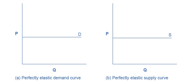
Perfectly elastic demand or supply implies that consumers or producers will only buy or sell at one price. A small change in price leads to an infinite change in quantity demanded or supplied.

Perfectly Elastic Demand

Perfectly elastic demand (elasticity = ∞) means that consumers will only buy at one price and any change in price will drop the quantity demanded to zero.

Case Study: Agricultural Commodities on the International Market

• Wheat exports from the United States.
• If the price of U.S. wheat is higher than the global market price, international buyers will switch to other suppliers like Canada or Australia.
• A slight increase in price results in a drastic drop in quantity demanded, demonstrating near-perfect elasticity.
• Agricultural commodities in highly competitive international markets exhibit nearly perfectly elastic demand as buyers have multiple alternative sources.

Perfectly Elastic Supply

Perfectly elastic supply (elasticity = ∞) means that suppliers will supply any quantity at a given price, but nothing at a different price.

Case Study: Digital Products and Services

• Software licenses and digital subscriptions.
• Companies like Microsoft can supply an infinite number of software licenses at a given price point.
• If the price drops below the threshold, suppliers may withdraw from the market entirely.
• The supply of digital products like software licenses is perfectly elastic, as firms can easily scale production to meet any level of demand at a set price.

Zero Elasticity

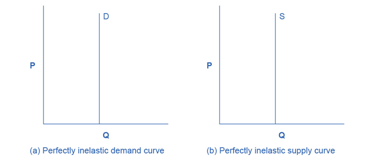
Perfectly inelastic demand or supply implies that quantity demanded or supplied is unaffected by any change in price.

 Perfectly Inelastic Demand

Perfectly inelastic demand (elasticity = 0) means that quantity demanded does not change, regardless of price changes.

Case Study: Life-Saving Medications in the United States

• Insulin for diabetes patients.
• Between 2002 and 2013, the price of insulin in the United States tripled.
• Despite the price surge, the quantity demanded remained largely unchanged because insulin is essential for survival.
• Life-saving medications like insulin have perfectly inelastic demand because patients need these medications regardless of price.

Perfectly Inelastic Supply

Perfectly inelastic supply (elasticity = 0) means that quantity supplied does not change regardless of price changes.

Case Study: Urban Land Supply in Tokyo

• Available land for construction in central Tokyo.
• The total supply of land is fixed, and cannot increase in response to rising prices.
• Despite high demand and skyrocketing prices, the quantity of land available for development remains constant.
• Urban land in highly populated cities like Tokyo has perfectly inelastic supply due to physical constraints.

Constant Unitary Elasticity

This is the case when the elasticity remains the same over a range of prices.

Constant Elasticity of Demand

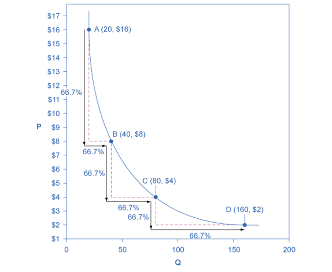
Constant elasticity of demand implies that the percentage change in quantity demanded is proportional to the percentage change in price.

Graphical Representation

In Figure 6.5, a demand curve with constant unit elasticity is depicted. Using the midpoint method, we find that between points A and B on the demand curve, both price and quantity demanded change by 66.7%. This results in an elasticity of 1. Similarly, between points B and C, and C and D, the percentage changes in price and quantity are also 66.7%, maintaining an elasticity of 1. It’s important to note that while the percentage declines in price vary as we move down the demand curve—$8.00 from A to B, $4.00 from B to C, and $2.00 from C to D—the elasticity remains constant at 1. This illustrates that a demand curve with constant unitary elasticity shifts from a steeper slope on the left to a flatter slope on the right, creating an overall curved shape.

Case Study: Luxury Cars in Europe

• The market for high-end vehicles like BMW and Mercedes-Benz.
• Studies show the price elasticity of demand for luxury cars in Europe is approximately -1, indicating unitary elasticity.
• A 10% increase in the price of luxury cars leads to a 10% decrease in the quantity demanded, and vice versa.
• The demand for luxury cars in Europe shows constant elasticity, meaning that the percentage change in price results in an equal percentage change in quantity demanded.

Constant Elasticity of Supply

Constant elasticity of supply implies that the percentage change in quantity supplied is proportional to the percentage change in price.

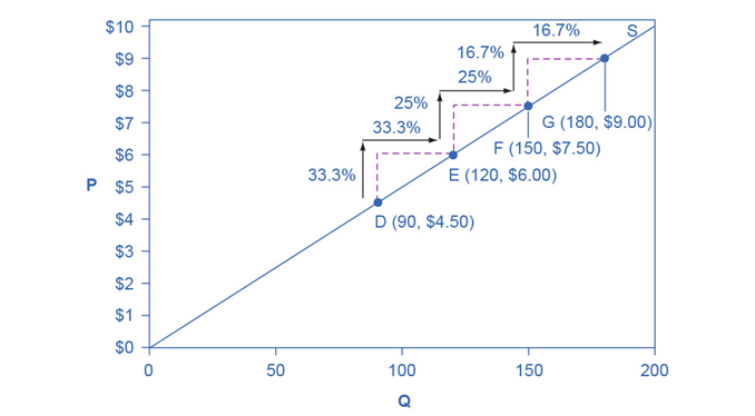
The supply curve with unitary elasticity is depicted as a straight line passing through the origin, unlike the demand curve with unitary elasticity which shows a curved shape. Each pair of points on this supply curve exhibits an equal difference in quantity, typically 30 units. However, when measured in percentage terms using the midpoint method, these steps decrease from 28.6% to 22.2% to 18.2% as we move from left to right along the curve. This reduction occurs because the quantity points used in each percentage calculation become progressively larger, thereby increasing the denominator in the elasticity formula for percentage change in quantity.

For instance, consider the price changes as we move upwards along the supply curve in Figure 6.6, from points D to E to F to G. Each step represents an absolute change of $1.50 in price. However, when measured in percentage terms using the midpoint method, these changes decrease from 28.6% to 22.2% to 18.2%. This pattern reflects the increasing original price points in each percentage calculation, thereby expanding the denominator in the calculation of percentage change in price.

Overall, the constant unitary elasticity supply curve maintains that the percentage changes in quantity along the horizontal axis exactly match the percentage changes in price along the vertical axis at all points.

Case Study: Oil Production in the Middle East

• Oil supply from Saudi Arabia.
• Research indicates that the price elasticity of supply for oil is relatively constant at around 0.5.
• A 10% increase in the price of oil leads to a 5% increase in quantity supplied.
• The supply of oil from major producers like Saudi Arabia shows constant elasticity, where changes in price result in proportional changes in supply.

---

Application of Elasticity Concepts in Real-World Scenarios

Elasticity and Pricing

Elasticity of demand and supply plays a crucial role in determining how prices adjust in response to changes in market conditions. Understanding elasticity helps businesses and policymakers make informed decisions about pricing strategies, production levels, and market interventions.

Case Study 1: Oil Prices and Elasticity

Oil prices are highly sensitive to changes in supply and demand due to their essential role in global energy markets. The elasticity of demand and supply for oil impacts how price changes affect consumption and production levels.

Example: During the COVID-19 pandemic in 2020, global oil demand dropped as lockdowns reduced travel and economic activity. The price of crude oil fell sharply, triggering responses from oil-producing nations to cut production to stabilize prices. For instance, in April 2020, the price of West Texas Intermediate (WTI) crude oil briefly turned negative for the first time, highlighting the extreme elasticity of demand and supply in the oil market.

• In April 2020, WTI crude oil prices fell to -$37.63 per barrel due to oversupply and plummeting demand.
• The pandemic-induced demand shock resulted in a 9.3% decrease in global oil demand for the year, according to the International Energy Agency (IEA).

Case Study 2: Elasticity in Airline Ticket Pricing

The airline industry faces elastic demand, particularly for leisure travel, where consumers can easily postpone or cancel trips based on price changes. This elasticity influences how airlines set ticket prices and manage revenues.

Example: Following the global financial crisis in 2008, airlines experienced a sharp decline in demand due to economic uncertainty and reduced consumer spending. To stimulate demand, airlines implemented dynamic pricing strategies, offering discounts and promotions to fill seats. This elasticity-driven pricing strategy helped airlines maintain cash flow during the economic downturn.

• In 2009, global airline passenger traffic declined by 2.9% compared to the previous year, according to the International Air Transport Association (IATA).
• Airlines adjusted ticket prices dynamically, resulting in a 6.5% decrease in average airfares to stimulate demand during the crisis.

Case Study 3: Elasticity in Consumer Electronics

Consumer electronics exhibit elastic demand due to rapid technological advancements, availability of substitutes, and varying consumer preferences. Changes in prices can significantly impact consumer purchasing decisions and market dynamics.

Example: The introduction of new smartphone models often triggers changes in demand elasticity within the consumer electronics market. Consumers may delay purchases or opt for cheaper alternatives when prices of flagship models increase.

• Apple Inc. faced elastic demand for its iPhone models in 2018 when it reported slower-than-expected sales of the iPhone X due to its high price tag.
• Price elasticity studies indicated that a 10% increase in iPhone prices led to a more than proportional decrease in sales volume, highlighting the sensitivity of demand to pricing changes in the smartphone market.

Raising Prices Raises Revenues or not?

Usually we think that companies earn high revenues with higher prices. But this is not the case actually. Understanding how changes in price affect total revenue based on the elasticity of demand is crucial for businesses and policymakers. Let’s explore the concepts of elastic, unitary, and inelastic demand and examine world around us to illustrate this phenomenon.

Elastic Demand and Falling Revenues:

Elastic Demand: When the percentage change in quantity demanded (% change in Qd) is greater than the percentage change in price (% change in P). Or % change in Qd > % change in P

Revenue Impact: A given percentage rise in price will be more than offset by a larger percentage fall in quantity demanded, causing total revenue (P × Q) to fall.

Case Study 1: Airline Tickets during Off-Peak Seasons

Airlines often lower ticket prices during off-peak seasons to attract more passengers. The demand for airline tickets is elastic during these periods because consumers are sensitive to price changes and have alternative modes of transportation or can choose to travel at different times.

A study by the International Air Transport Association (IATA) showed that a 10% reduction in ticket prices during off-peak seasons led to a 15% increase in passengers.

Case Study 2: Luxury Goods Market

The demand for luxury goods such as high-end watches and designer handbags is highly elastic. Consumers are sensitive to price changes and may defer purchases or opt for less expensive alternatives when prices rise.

According to a report by Bain & Company, a 5% increase in the prices of luxury watches resulted in an 8% decline in sales volume.

Case Study 3: Movie Theaters

Movie theaters often experience elastic demand. Consumers have multiple entertainment options, and a slight increase in ticket prices can lead to a significant drop in attendance.

A survey by the National Association of Theatre Owners found that a 10% increase in ticket prices led to a 12% decrease in moviegoers.

Unitary Elastic Demand and Unchanged Revenues

Unitary Elastic Demand: When the percentage change in quantity demanded (% change in Qd) is equal to the percentage change in price (% change in P).

Revenue Impact: A given percentage rise in price will be exactly offset by an equal percentage fall in quantity demanded, keeping total revenue (P × Q) unchanged.

Case Study 1: Telecom Services in Competitive Markets

In highly competitive telecom markets, price changes by one provider are often matched by changes in consumer usage, leading to unitary elastic demand.

In India, a study showed that a 5% increase in data plan prices led to a 5% decrease in data usage, keeping overall revenue constant.

Case Study 2: Fast Food Industry

The fast food industry often sees unitary elastic demand, where price changes lead to proportional changes in quantity demanded.

A McKinsey report indicated that a 3% increase in the price of a popular meal combo resulted in a 3% decrease in sales volume, leaving revenue unchanged.

Case Study 3: Public Transportation

Public transportation systems in cities with multiple commuting options can experience unitary elastic demand.

In Hong Kong, a 2% increase in subway fares led to a 2% decrease in ridership, maintaining total fare revenue.

Inelastic Demand and Increasing Revenues

Inelastic Demand: When the percentage change in quantity demanded (% change in Qd) is less than the percentage change in price (% change in P).

Revenue Impact: A given percentage rise in price will cause a smaller percentage fall in quantity demanded, resulting in an increase in total revenue (P × Q).

Case Study 1: Essential Medicines

The demand for essential medicines, such as insulin, is inelastic. Patients need these medications regardless of price changes.

A study published in the Journal of Health Economics showed that a 10% increase in the price of insulin resulted in only a 2% decrease in quantity demanded, increasing overall revenue for pharmaceutical companies.

Case Study 2: Basic Utilities

Basic utilities like electricity and water have inelastic demand because consumers cannot easily reduce usage in response to price hikes.

In the UK, a 5% increase in electricity prices led to a 1% decrease in consumption, increasing total revenue for utility providers.

Case Study 3: Cigarettes

The demand for cigarettes is relatively inelastic due to addiction. Even significant price increases do not lead to a proportionate decrease in quantity demanded.

According to the World Health Organization, a 20% increase in cigarette prices in Australia resulted in only a 5% decrease in sales, significantly boosting tax revenue.

Elasticity of Supply Curve and Their Impact on Revenues

Understanding the different types of elasticity of supply is crucial for businesses and policymakers. It helps predict how changes in price will impact the quantity supplied and, consequently, revenue. As the price increases more than the quantity supplied, revenue increases.

Elastic Supply and Higher Revenues

Elastic Supply: When the percentage change in quantity supplied (% change in Qs) is greater than the percentage change in price (% change in P). If demand is strong and the market can absorb the additional supply, revenue will increase.

Revenue Impact: When supply is elastic, a given percentage increase in price will result in a larger percentage increase in quantity supplied. This generally leads to higher total revenue, provided demand remains strong.

Case Study: Agricultural Products in the USA

Farmers can quickly increase the supply of crops in response to price changes by planting more or using advanced farming techniques.

During a period of high corn prices in the USA, a 15% increase in the price of corn led to a 20% increase in the quantity supplied due to the adoption of genetically modified seeds and improved irrigation systems. This increase in supply resulted in higher overall revenue for farmers.

Unitary Elastic Supply and Unchanged Revenues

Unitary Elastic Supply: When the percentage change in quantity supplied (% change in Qs) is equal to the percentage change in price (% change in P). This is a likely scenario as the percentage changes in price and quantity supplied are equal.

Revenue Impact: When supply is unitary elastic, a given percentage increase in price will result in an equal percentage increase in quantity supplied. Total revenue remains unchanged.

Case Study: Dairy Industry in New Zealand

Dairy farmers can adjust their milk production to match price changes due to efficient farming practices and technology.

In New Zealand, a 7% increase in milk prices resulted in a 7% increase in milk production, leading to unchanged total revenue.

Inelastic Supply and Higher Revenues

Inelastic Supply: When the percentage change in quantity supplied (% change in Qs) is less than the percentage change in price (% change in P).

Revenue Impact: When supply is inelastic, a given percentage increase in price will result in a smaller percentage increase in quantity supplied. This typically leads to higher total revenue.

Case Study: Oil Production in Saudi Arabia

The supply of oil is relatively inelastic due to the high cost and long time required to increase production capacity.

A 20% increase in global oil prices resulted in only a 5% increase in oil production from Saudi Arabia, leading to a significant rise in total revenue for the country.

---

Can Company Transfer Increased Costs to Consumers?

Most companies constantly look for ways to reduce production costs to earn higher revenues. However, sometimes the cost of essential inputs, which companies cannot control, increases. For example, chemical companies rely on petroleum, but they cannot control crude oil prices. Similarly, coffee shops need coffee but cannot influence global coffee prices. When these input costs rise, can companies pass the higher costs to consumers through increased prices? Conversely, when new, cheaper production methods are discovered, can companies keep the extra profits, or will market forces push them to lower prices for consumers? The price elasticity of demand helps answer these questions.

Passing along Cost Savings to Consumers

Elasticity of demand measures how sensitive the quantity demanded of a good is to a change in its price. If demand is elastic, a small price increase will lead to a significant drop in quantity demanded. If demand is inelastic, a price increase will lead to a small drop in quantity demanded.

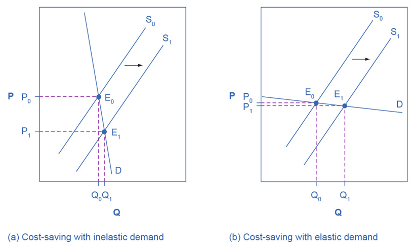
When a technological breakthrough makes production cheaper, it impacts consumers based on the demand elasticity. If the demand for a product is inelastic, as shown in Figure 6.7(a), a cost-saving improvement will significantly lower prices with little change in quantity sold. Conversely, if demand is elastic, as shown in Figure 6.7(b), the improvement leads to a substantial increase in quantity sold with minimal price reduction. Therefore, consumers benefit more in terms of price reduction when demand is inelastic.

Case Study 1: Technological Advancements in Smartphone Production

• In the mid-2010s, advances in technology significantly reduced the cost of producing smartphones.
• Impact on Smartphone Manufacturers: The cost of components like processors and memory dropped.
• Elasticity of Demand: The demand for smartphones is relatively elastic due to numerous substitutes and rapid technological advancements.
• Outcome: Competition among smartphone manufacturers led to lower prices for consumers rather than increased profits for producers. The technological savings were largely passed on to consumers, increasing the quantity demanded.

Case Study 2: Advances in Manufacturing of LED TVs

During the early 2010s, improvements in LED TV manufacturing processes significantly reduced production costs.

Impact on TV Manufacturers: Reduced costs for components and assembly.

Elasticity of Demand: The demand for LED TVs is relatively elastic due to the availability of substitutes and rapid technological changes.

Outcome: Manufacturers passed on the cost savings to consumers, resulting in lower retail prices and a significant increase in sales volume.

Case Study 3: Increased Efficiency in Car Manufacturing

In the late 2010s, car manufacturers adopted more efficient production techniques and automation.

Impact on Car Manufacturers: Lowered production costs.

Elasticity of Demand: The demand for cars is relatively elastic, as consumers have numerous alternatives and are sensitive to price changes.

Outcome: The savings from increased efficiency led to lower car prices, stimulating demand and boosting overall sales.

Passing along Higher Costs to Consumers

Companies constantly strive to lower production costs to increase profits. However, when the price of a key input, over which the business has no control, rises, they face a dilemma. Can they pass these higher costs on to consumers through higher prices? Conversely, if production costs decrease due to technological advances, can businesses retain the extra profits, or will market competition force them to lower prices? The price elasticity of demand plays a crucial role in answering these questions.

Figure 6.8 Passing along Cost Savings to Consumers

When taxes on cigarette producers increase, the supply curve shifts left, leading to higher consumer prices P1, as shown in Figure 6.8(a). Due to inelastic demand, this results in minimal reduction in smoking and higher tax revenue. To reduce smoking effectively, demand needs to shift left through public programs. Conversely, in Figure 6.8(b), with elastic demand, increased taxes significantly reduce smoking, especially among youth, who respond more to price changes than adults.

Case Study 1: Rising Oil Prices and the Airline Industry

In 2008, the global price of crude oil spiked, reaching over $140 per barrel.

Impact on Airlines: The airline industry, which relies heavily on fuel, faced significantly higher operating costs.

Elasticity of Demand: The demand for air travel is relatively elastic, as consumers can opt for alternative modes of transportation or choose not to travel.

Outcome: Airlines struggled to pass the entire increase in fuel costs to consumers through higher ticket prices. The higher costs led to reduced profitability and some airlines cutting routes or going bankrupt.

Case Study 2: Coffee Price Surge and Coffee Shops

In 2011, adverse weather conditions in major coffee-producing countries led to a significant increase in coffee prices.

Impact on Coffee Shops: Coffee shops faced higher costs for their primary input.

Elasticity of Demand: The demand for coffee is relatively inelastic, as many consumers consider coffee a necessity and have few substitutes.

Outcome: Coffee shops were able to pass on most of the increased costs to consumers through higher prices without a significant drop in sales.

Case Study 3: Pharmaceutical Industry and Raw Material Costs

In 2020, the price of raw materials for drug manufacturing surged due to supply chain disruptions during the COVID-19 pandemic.

Impact on Pharmaceutical Companies: Increased costs for essential raw materials.

Elasticity of Demand: The demand for pharmaceutical products is generally inelastic, as these products are often necessities with few substitutes.

 Outcome: Pharmaceutical companies passed on the higher costs to consumers through increased drug prices. Despite the higher prices, the quantity demanded remained relatively stable due to the necessity of these products.

Elasticity and Tax Incidence

Understanding how elasticity impacts tax incidence is crucial for both businesses and policymakers. Tax incidence refers to the distribution of the tax burden between buyers and sellers. The elasticity of demand and supply plays a key role in determining who bears the greater burden of a tax.

The Concept of Tax Incidence

Tax incidence describes how the burden of a tax is distributed between producers and consumers. When a tax is imposed on a good or service, the price usually increases for consumers and the revenue received by producers decreases. The extent to which these price changes affect consumers and producers depends on the elasticity of demand and supply.

Elasticity of Demand and Supply

Elastic Demand: When the demand for a product is elastic, consumers are very responsive to price changes. A small increase in price results in a significant decrease in quantity demanded.

Inelastic Demand: When demand is inelastic, consumers are less responsive to price changes. A price increase results in a relatively small decrease in quantity demanded.

Elastic Supply: Producers can easily change the quantity they supply in response to price changes.

Inelastic Supply: Producers are less able to change the quantity they supply in response to price changes.

Tax Burden Distribution

Tax on Inelastic Demand: When demand is inelastic, consumers bear a larger portion of the tax burden because they are less responsive to price increases.

Tax on Elastic Demand: When demand is elastic, producers bear a larger portion of the tax burden because consumers will significantly reduce their quantity demanded if prices increase.

Tax on Inelastic Supply: When supply is inelastic, producers bear a larger portion of the tax burden because they cannot easily reduce the quantity they supply.

Tax on Elastic Supply: When supply is elastic, consumers bear a larger portion of the tax burden because producers can easily reduce the quantity they supply if the price decreases.

Graphical Representation of Elasticity and Tax Incidence

An excise tax creates a gap between the price consumers pay (Pc) and the price producers receive (Pp). This gap equals the tax per unit. Pe represents the equilibrium price before the tax is imposed. The incidence of the tax—the distribution of the tax burden between consumers and producers—depends on the relative elasticities of demand and supply.

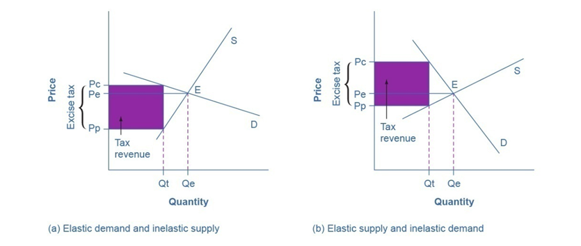
Figure 6.9 Elasticity and Tax Incidence

(a) Demand Is More Elastic than Supply:

• When demand is more elastic than supply, consumers are more responsive to price changes than producers.
• Tax incidence on consumers (Pc – Pe) is smaller than on producers (Pe – Pp).
• Example: Beachfront hotels, where consumers have alternatives, but sellers cannot easily relocate.
• Tax revenue is lower because the elastic demand reduces the quantity sold significantly when prices increase.

(b) Supply Is More Elastic than Demand:

• When supply is more elastic than demand, producers are more responsive to price changes than consumers.
• Tax incidence on consumers (Pc – Pe) is larger than on producers (Pe – Pp).
• Example: Tobacco excise tax, where consumers have fewer alternatives, but producers can adjust their quantities more easily.
• Tax revenue is higher because the inelastic demand means consumers do not reduce their quantity demanded as much when prices increase.

Key Points:

• The tax burden falls more on the less elastic side of the market.
• The more elastic the demand and supply curves, the lower the tax revenue because both consumers and producers reduce their quantities significantly in response to price changes.
• Inelastic Supply, Elastic Demand (Figure 6.9a): Larger tax burden on producers.
• Elastic Supply, Inelastic Demand (Figure 6.9b): Larger tax burden on consumers.

World around Us: Tax Incidence

Case Study 1: Cigarette Tax in the United States

Context: The US government imposes high taxes on cigarettes to reduce smoking and increase government revenue.

Facts and Figures: According to the Centers for Disease Control and Prevention (CDC), federal and state taxes on cigarettes vary, but the average state tax in 2021 was about $1.91 per pack.

Analysis: Cigarette demand is relatively inelastic because nicotine is addictive. As a result, consumers bear a larger portion of the tax burden. Despite higher prices, the reduction in quantity demanded is relatively small. The tax effectively reduces smoking rates but also generates substantial revenue for the government.

Case Study 2: Fuel Taxes in the European Union

Context: Many European countries impose high taxes on fuel to encourage the use of public transportation and reduce carbon emissions.

Facts and Figures: In 2022, the average fuel tax in the EU was around €0.60 per liter, varying significantly between member states.

Analysis: Fuel demand is relatively inelastic because there are few immediate substitutes for car travel, especially in rural areas. Consequently, consumers bear most of the tax burden. High fuel taxes have led to increased revenue for governments and a modest reduction in fuel consumption, contributing to environmental goals.

Case Study 3: Luxury Goods Tax in India

Context: The Indian government imposes high taxes on luxury goods to generate revenue and reduce wealth inequality.

Facts and Figures: In 2018, luxury cars in India faced a Goods and Services Tax (GST) rate of 28%, plus an additional cess of up to 22%.

Analysis: The demand for luxury goods is more elastic because they are non-essential and have many substitutes. Therefore, producers bear a significant portion of the tax burden. High taxes have led to a decrease in the quantity demanded of luxury goods, as consumers opt for cheaper alternatives or delay their purchases.

Understanding the interplay between elasticity and tax incidence is vital for effective tax policy. Policymakers need to consider how the elasticity of demand and supply will influence who bears the tax burden. Through these case studies, we see that the elasticity of the product significantly affects how taxes impact prices, quantities, and overall economic welfare. Effective tax policy requires a nuanced understanding of these economic principles to achieve desired outcomes without unintended consequences.

---

Long-Run vs. Short-Run Impact of Elasticities

Elasticities are often lower in the short run than in the long run due to the limited time available for consumers and producers to adjust their behaviors and capacities.

Aspect	Short-Run Impact	Long-Run Impact
Price Elasticity of Demand	Lower; consumers have less time to adjust to price changes	Higher; consumers have more time to find substitutes or change consumption habits
Price Elasticity of Supply	Lower; producers cannot quickly change production levels	Higher; producers can adjust production levels and capacity
Revenue Impact	Less responsive; smaller changes in quantity demanded/supplied	More responsive; larger changes in quantity demanded/supplied
Examples	Gasoline demand, housing supply	Electric cars demand, renewable energy supply

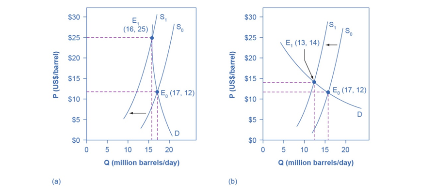
Figure 6.10 Long Run vs. Short Run Impacts 

In 1973, a shift in the supply of crude oil due to OPEC’s embargo led to a significant increase in oil prices in the U.S. Figures 6.10(a) and (b) show the impact of this supply shift with different demand elasticities:

• Figure 6.10(a): Inelastic demand results in a significant price increase (from $12 to $25 per barrel) with a small decrease in quantity (from 17 to 16 million barrels per day).
• Figure 6.10(b): Elastic demand results in a smaller price increase (to $14 per barrel) and a larger decrease in quantity (to 13 million barrels per day).

Long Run Impact:

Over the long term, demand for oil became more elastic, leading to reduced consumption despite economic growth, as evidenced by the U.S. in 1983. This gradual reduction in oil consumption, especially in the U.S., can be attributed to several factors:

1. Conservation Efforts: High oil prices spurred initiatives to reduce energy usage, including government policies and public awareness campaigns.
2. Technological Advances: Development and adoption of more fuel-efficient vehicles, machinery, and appliances.
3. Alternative Energy Sources: Increased research and use of alternative energy sources reduced reliance on oil.
4. Economic Adaptations: Industries adapted by optimizing processes to be less energy-intensive.

These efforts collectively increased the elasticity of demand for oil, leading to a more significant reduction in oil consumption over time despite economic growth.

---

Some Other Forms of Elasticities other than Price

1. Income Elasticity of Demand (YED)
2. Cross-Price Elasticity of Demand (XED)
3. Elasticity in Labor Market
4. Elasticity in Financial Market

Income Elasticity of Demand

Income Elasticity of Demand (YED) measures how the quantity demanded of a good responds to changes in consumer income. The formula for calculating YED is:

World around Us: Income Elasticity of Demand

Case Study 1: Luxury Cars

Scenario: Economic Boom in China

Context: In recent years, China’s burgeoning middle and upper class has significantly increased.

Facts: Between 2010 and 2020, China’s GDP per capita grew from approximately $4,550 to $10,276.

Figures: Sales of luxury cars like BMW and Mercedes-Benz surged, with BMW’s sales increasing by 36% from 2019 to 2020.

YED: The high income elasticity (YED > 1) for luxury cars indicates they are luxury goods.

Case Study 2: Basic Food Items

Scenario: Economic Downturn in the U.S.

Context: During the 2008 financial crisis, many households experienced reduced incomes.

Facts: Incomes fell by about 6% on average.

Figures: Despite the income drop, the demand for staple foods like bread and milk remained relatively stable, increasing by about 2%.

YED: The low positive YED (< 1) for staple foods shows they are necessities.

Case Study 3: Public Transportation

Scenario: Post-Recession Recovery in Spain

Context: Following the European debt crisis, Spain’s economy began to recover slowly.

Facts: From 2014 to 2019, Spain’s GDP per capita grew from $28,315 to $30,370.

Figures: Use of public transportation decreased by 5% as more people could afford private vehicles.

YED: The negative YED (< 0) for public transportation signifies it is considered an inferior good/commodity during economic recovery.

Cross-Price Elasticity of Demand (XED)

Cross-Price Elasticity of Demand (XED) measures the responsiveness of the quantity demanded for one good when the price of another good changes. The formula for calculating XED is:

World around Us: Cross-Price Elasticity of Demand (XED)

Case Study 1: Coca-Cola and Pepsi

Scenario: Competitive Pricing in the Beverage Industry

Context: Coca-Cola and Pepsi are direct competitors in the soft drink market.

Facts: When Pepsi increased its price by 10% in 2019, Coca-Cola saw a 5% increase in its sales.

Figures: XED calculation indicates a positive value, suggesting that Coca-Cola and Pepsi are substitute goods.

XED: Approximately +0.5 (indicating substitution effect).

Case Study 2: Printers and Ink Cartridges

Scenario: Pricing Strategies in the Technology Market

Context: Printers and ink cartridges are complementary goods.

Facts: A 15% decrease in the price of printers led to a 20% increase in the demand for ink cartridges in 2020.

Figures: The XED for printers and ink cartridges is negative, reflecting their complementary nature.

XED: Approximately -1.33 (indicating complementarities).

Case Study 3: Gasoline and Public Transportation

Scenario: Fluctuating Fuel Prices and Commuter Behavior

Context: Gasoline and public transportation are considered substitutes to some extent.

Facts: In 2018, a 20% increase in gasoline prices resulted in a 10% increase in public transportation usage in urban areas.

Figures: This positive XED shows that public transportation is a substitute for gasoline for some commuters.

XED: Approximately +0.5 (indicating substitution effect).

Elasticity in the Labor Market

Elasticity in the labor market refers to how sensitive the supply and demand for labor is to changes in wages or other economic variables. There are two main types of labor market elasticity: wage elasticity of labor supply and wage elasticity of labor demand.

World around Us: Elasticity in Labor Market

Case Study 1: Minimum Wage Increase in Seattle

Context: In 2014, Seattle implemented a phased increase in the minimum wage, reaching $15 per hour by 2021.

Facts: Studies showed a mixed response in labor supply and demand. Low-wage workers saw increased earnings, but some small businesses reduced their hiring or hours to offset higher wage costs.

Figures: A study by the University of Washington found that a 10% increase in the minimum wage led to a 1% reduction in hours worked for low-wage workers.

Elasticity: Wage elasticity of labor demand for low-wage workers, was found to be -0.1, indicating relatively inelastic demand.

Case Study 2: Tech Industry Boom in Silicon Valley

Context: The rapid growth of the tech industry in Silicon Valley increased the demand for skilled labor, leading to rising wages.

Facts: Between 2010 and 2020, wages for software developers increased by 50%, while the quantity of labor supplied increased by 30%.

Figures: The influx of skilled workers from other regions and countries significantly contributed to the labor supply.

Elasticity: Wage elasticity of labor supply for software developers was calculated as 0.6, indicating a moderately elastic supply.

Case Study 3: Agricultural Labor Market and Immigration Policies

Context: Changes in U.S. immigration policies have affected the supply of migrant labor in agriculture.

Facts: Stricter immigration enforcement in the 2010s reduced the availability of migrant labor, leading to higher wages for remaining workers but also labor shortages in some areas.

Figures: A 20% reduction in migrant labor availability led to a 10% increase in wages for agricultural workers.

Elasticity: Wage elasticity of labor supply was -0.5, indicating inelastic supply.

Elasticity in Financial Capital Markets

Elasticity in financial and capital markets measures how responsive the supply and demand for financial instruments is to changes in various economic factors, such as interest rates or stock prices. The two primary elasticities are interest rate elasticity of investment and price elasticity of demand for financial assets. The savings and borrowings also exhibit elastic properties.

a. Interest Rate Elasticity of Investment

Case Study: U.S. Federal Reserve Interest Rate Cuts (2008-2009)

Context: During the financial crisis of 2008-2009, the U.S. Federal Reserve significantly cut interest rates to stimulate the economy.

Facts: The Federal Reserve reduced the federal funds rate from 5.25% in 2007 to nearly 0% by the end of 2008.

Figures: Investment in new housing and business equipment increased by approximately 20% as borrowing costs fell.

Elasticity: The interest rate elasticity of investment was calculated to be around -2.0, indicating high sensitivity to interest rate changes.

b. Price Elasticity of Demand for Financial Assets

Case Study: Stock Market Reaction to COVID-19 Pandemic (2020)

Context: The outbreak of COVID-19 in early 2020 caused significant volatility in global stock markets.

Facts: The S&P 500 index fell by approximately 34% from February to March 2020 due to pandemic fears.

Figures: The demand for safe-haven assets like U.S. Treasury bonds surged, with bond yields dropping to historic lows.

Elasticity: The price elasticity of demand for U.S. Treasury bonds was estimated to be -1.5, showing substantial responsiveness to changes in stock market conditions.

Elasticity of Savings

The elasticity of savings measures how responsive the amount of savings is to changes in economic factors such as interest rates.

Case Study: U.S. Personal Savings Rate during the COVID-19 Pandemic

Context: The economic uncertainty during the COVID-19 pandemic led to changes in savings behavior in the United States.

Facts: The U.S. personal savings rate soared from 7.6% in January 2020 to 33.8% in April 2020 (Bureau of Economic Analysis). Interest rates were reduced to near zero by the Federal Reserve.

Figures: Personal savings rose from $1.4 trillion to $6.4 trillion. Despite low-interest rates, the high savings rate suggests a low elasticity of savings, indicating that economic uncertainty played a significant role.

Elasticity of Borrowings

The elasticity of borrowings measures how approachable the amount of borrowing is when the interest rates are changed.

Case Study: U.S. Mortgage Borrowing during Housing Boom

Context: The U.S. housing boom in the early 2000s saw significant changes in borrowing behavior influenced by interest rates.

Facts: Interest rates were reduced from 6.5% in 2000 to 1% in 2003 by the Federal Reserve. Mortgage borrowing increased substantially during this period.

Figures: Total mortgage debt rose from $4.94 trillion in 2000 to $8.94 trillion in 2004 (Federal Reserve). The sharp rise in borrowing despite falling interest rates indicates a high elasticity of borrowing, where lower interest rates led to a significant increase in the quantity of borrowings.

---

Importance of Understanding Elasticity

By mastering the concepts of price elasticity of demand and supply, we can better predict market responses, design effective policies, and optimize pricing strategies. Elasticity not only helps in understanding past market behaviors but also in forecasting future trends and making strategic decisions.

Pricing Strategies

• Businesses: Knowing the price elasticity of demand for their products helps businesses set optimal prices. For example, if demand is elastic, a small price increase could lead to a significant drop in sales, so businesses might avoid raising prices. Conversely, if demand is inelastic, businesses can raise prices with minimal impact on the quantity sold, increasing their revenue.
• Governments: Understanding elasticity helps in setting taxes. For goods with inelastic demand (like tobacco), higher taxes can reduce consumption without significantly decreasing tax revenue.

Revenue and Profit

• Revenue Calculation: Elasticity impacts how price changes affect total revenue. For elastic goods, a price decrease can increase total revenue, whereas, for inelastic goods, a price increase can increase total revenue.
• Profit Maximization: Businesses can use elasticity data to determine the most profitable price point. If a company knows its product’s elasticity, it can better predict how changes in price will affect its overall profit margins.

Policy Making

• Taxation: Governments use elasticity to predict how taxes will affect market behavior. For example, taxes on inelastic goods like alcohol or cigarettes are less likely to decrease consumption significantly but can generate substantial revenue.
• Subsidies and Price Controls: Policies such as rent control or minimum wage laws can be better designed with an understanding of elasticity. For instance, if the supply of housing is inelastic, rent control might lead to severe shortages.

---

Elasticity through the Lens of Behavioral Economics

Elasticity refers to how sensitive the quantity demanded or supplied of a good is to changes in price, income, or other factors. Traditional economics assumes that consumers and firms make decisions based on rational calculations of costs and benefits. However, behavioral economics reveals that people’s decisions often deviate from rational models due to psychological biases, emotions, and social factors.

Scenario: Price Elasticity of Demand for a Luxury Brand

A luxury clothing brand increases its prices by 20%, assuming that the high-income target market will continue purchasing at the same rate. Traditional economics would predict that if the demand is inelastic, the quantity demanded would only decrease slightly, as high-income consumers are less sensitive to price changes.

However, behavioral economics highlights that consumer behavior is influenced by more than just price. Cognitive biases and social factors play a significant role.

Cognitive Biases:

Many consumers experience status quo bias, preferring to stick with their habitual luxury brand purchases, even at higher prices. But loss aversion may also come into play—consumers are more sensitive to the perceived loss of wealth from paying more for the same product, leading to a sharper decrease in demand than traditional models predict.

Social Influence:

The bandwagon effect can cause consumers to continue purchasing luxury goods despite price increases if they perceive that others in their social group are still buying the product. Conversely, if consumers see their peers moving away from the brand due to price hikes, they may follow suit, making demand more elastic than expected.

The “bandwagon effect” refers to the tendency of people to adopt a behavior, style, or attitude simply because others are doing it. It’s like following the crowd—if many people start doing something, others are likely to join in, often without much thought, just because it seems popular.

Facts and Figures:

Research shows that when price increases are combined with effective marketing that highlights exclusivity or scarcity (like limited-edition releases), the demand elasticity for luxury goods decreases. In a study of luxury watch brands, price increases of up to 30% led to only a 10% drop in sales, as the brand managed to reinforce its exclusive image.

Summary

Behavioral economics suggests that factors such as loss aversion, social influence, and the framing of price changes significantly impact the elasticity of demand, particularly in markets for luxury goods. This case study demonstrates how psychological and social factors must be considered alongside traditional economic models.

---

Research Suggestions for Economists in Behavioral Economics

The rising population is worsening the economic conditions in Pakistan. The behavioral economics can better understand the prefrences shifts. Below are few suggestions to reach some feasible solutions to our problems.

1. Academic Journals: Look for studies published in journals related to marketing, consumer behavior, or economics. Journals like the Journal of Consumer Research or the Journal of Marketing might have relevant studies on luxury goods and price elasticity.
2. Industry Reports: Reports from consulting firms like McKinsey, Bain & Company, or Deloitte often provide insights into luxury markets and consumer behavior.
3. Case Studies: Refer to specific case studies on luxury brands that have implemented price increases. These might be found in business school case collections or books focused on luxury brand management.
4. Books: Books like “Luxury Marketing: A Challenge for Theory and Practice” by Klaus-Peter Wiedmann and Nadine Hennigs often contain detailed studies and references to real-world examples.
5. Impact of Loss Aversion on Price Elasticity: Investigate how loss aversion affects consumers’ responses to price changes in various markets, particularly for essential goods versus luxury goods.
6. Framing Effects and Elasticity: Study how different ways of presenting price increases (e.g., emphasizing quality improvements or exclusive benefits) impact consumer elasticity across different income groups
7. Social Influence on Demand Elasticity: Explore how social media and peer influence shape the elasticity of demand in fashion, tech gadgets, and other trend-driven markets.
8. Nudging and Price Sensitivity: Analyze how small nudges, such as loyalty rewards or small discounts, affect the price sensitivity of consumers in the context of price elasticity.

These research directions provide valuable insights into how behavioral factors shape real-world economic outcomes beyond traditional elasticity models.

---

Critical Thinking

1. How does understanding elasticity help businesses make pricing decisions?
2. Explain how elasticity affects total revenue when prices are increased or decreased.
3. Why might the elasticity of savings be lower during times of economic uncertainty?
4. How can changes in interest rates influence individual saving behaviors differently based on the economic context?
5. What factors can cause the elasticity of borrowing to change over time?
6. Why did the U.S. mortgage borrowing increase substantially during the early 2000s despite falling interest rates?
7. How does the elasticity of demand and supply influence the incidence of taxation on consumers and producers?
8. What are the potential policy implications if the demand for a good is highly inelastic when taxes are imposed?
9. Why elasticities are often lower in the short run compared to the long run? Provide an example to support your answer.
10. How might businesses and consumers adjust differently to price changes in the short run versus the long run?
11. During the COVID-19 pandemic, the U.S. personal savings rate increased significantly despite low-interest rates. What does this suggest about the elasticity of savings during that period?
12. The OPEC oil embargo in 1973 led to different outcomes depending on the elasticity of demand. How did the short-run and long-run responses to the embargo differ in the U.S.?
13. How can policymakers use knowledge of elasticity to design effective economic policies?
14. Consider a good with inelastic demand, like gasoline. How might a sudden supply shock affect prices and quantities in the market?
15. How can businesses use cross-price elasticity to develop competitive pricing strategies in markets with many substitute goods?
16.  Discuss how cross-price elasticity can inform decisions about bundling products.