Today, we will explore one of the fundamental concepts in economics: Demand and Supply. Understanding these concepts is crucial for analyzing how markets function at the individual level and on a larger scale. We will discuss how demand and supply interact to determine prices and quantities in markets, factors that cause shifts in demand and supply, and how these shifts affect market equilibrium. We will also look at price ceilings and price floors, and their impact on market efficiency.
Demand and Supply in Markets for Goods and Services
We will start our discussion on demand and supply concepts with a simple and relatable example: ” The low-priced products is a fascinating concept but inaccessible“. We all know environmentally friendly products are often more costly and there are forces that resist lowering their prices. This issue has significant implications for consumers, businesses, and the environment.
Reasons for the Higher Cost of Environmentally Friendly Products
- Higher Production Costs
Environmentally friendly products often involve more expensive raw materials and sustainable production processes. These costs are passed on to consumers. Organic vegetables cost more than conventionally grown ones because organic farming avoids synthetic pesticides and fertilizers, which increases labor and land use.
- Economies of Scale
Many environmentally friendly products are produced on a smaller scale compared to their conventional counterparts. This means they cannot benefit from the cost savings associated with large-scale production. We will discuss this concept in detail in the upcoming lectures.
For example, electric cars are generally more expensive than gasoline cars partly because they are produced in smaller quantities. As production increases, costs are expected to come down.
- Research and Development Costs
Developing new environmentally friendly technologies and products requires significant investment in research and development (R&D). These R&D costs are reflected in the price of the products.
For example, solar panels were initially very expensive due to high R&D costs. Although prices have decreased over time, they are still more costly compared to conventional energy sources in many regions.
Forces Resisting the Lowering of Prices
- Market Demand and Consumer Willingness to Pay
While there is growing demand for green products, it is not yet at a level where mass production can drive down costs significantly. Additionally, consumers may not be willing to pay a premium for environmentally friendly options. Or you can say that the most of the consumers do not have enough purchasing power to afford these products.
Biodegradable plastics are more expensive than regular plastics because the demand, although growing, is not yet sufficient to achieve significant economies of scale.
- Government Policies and Subsidies
Many conventional industries receive subsidies and favorable policies that environmentally friendly industries do not. This creates an uneven playing field and keeps prices of green products high.
For example, fossil fuel industries often receive substantial subsidies, making gasoline cheaper than renewable energy options like wind or solar power. The IPPs (Independent Power Producers) in Pakistan can be the case study for researchers.
- Existing Infrastructure and Technology
The current infrastructure and technology are often geared towards conventional products. Transitioning to environmentally friendly alternatives requires substantial investment in new infrastructure, which keeps costs high.
For example, the widespread availability of gas stations and the existing automobile industry’s focus on internal combustion engines make it challenging for electric vehicles to compete on price without significant investment in new infrastructure for charging stations.
World Around Us: Environment-Friendly Products
- Reusable Shopping Bags vs. Plastic Bags
Reusable shopping bags are typically more expensive than plastic bags. The higher cost is due to better materials and more durable construction. However, plastic bags are cheaper because they are produced in massive quantities and benefit from economies of scale.
Forces resisting price reduction: Lack of strong regulatory measures to phase out plastic bags, higher initial investment for reusable bags, and consumer reluctance to change habits.
- Energy-Efficient Appliances vs. Standard Appliances
Energy-efficient appliances like LED light bulbs, refrigerators, and washing machines often cost more upfront than standard models. The higher cost is due to advanced technology and materials that reduce energy consumption.
Forces resisting price reduction: Existing manufacturing processes and supply chains optimized for standard appliances, lack of consumer awareness, and initial higher investment costs for energy-efficient technologies.
- Organic Food vs. Conventional Food
Organic foods are usually more expensive than conventionally grown foods. The reasons include more labor-intensive farming practices, higher land costs, and lower yields per acre.
Forces resisting price reduction: Large-scale industrial farming of conventional crops, subsidies for conventional farming, and consumer price sensitivity.
The researchers must explore these dimensions,” Corporate Agriculture Farming: Advantages and Disadvantages” and “Corporate Agriculture Farming is a Solution to the Global Hunger Crisis”.
Understanding why environmentally friendly products are costly and what forces resist lowering their prices is crucial for making informed decisions as consumers and policymakers. While these products often have higher initial costs, their long-term benefits to the environment and health can be significant. As demand increases and technology advances, we can hope to see a reduction in their prices, making them more accessible to everyone.
What is Demand?
Demand refers to the quantity of a good or service that consumers are willing and able to purchase at various prices over a given period. The demand curve shows the relationship between the price of a good and the quantity demanded.
Example: Think about your consumption of fruits. If the price of apples decreases, you might buy more apples. Conversely, if the price increases, you might buy fewer apples. This illustrates the law of demand: as the price of a good falls, the quantity demanded rises, and vice versa.
Factors Affecting Demand
- Income: Higher income generally increases demand for goods.
- Prices of Related Goods: The demand for a good can be affected by the prices of substitutes and complements.
- Tastes and Preferences: Changes in consumer preferences can shift demand.
- Expectations: If people expect prices to rise in the future, they might buy more now.
Graphing Demand Curves and Shifts
A demand curve slopes downward from left to right. An increase in demand shifts the curve to the right; a decrease shifts it to the left. In the Smartphone market, if a new model becomes very popular, the demand for that model will increase, shifting the demand curve to the right.
Demand Schedule
A demand schedule is a table that shows how many units of a good or service people are willing to buy at different prices. For example, Table 3.1 shows the quantity of gasoline demanded at various prices.
Table 3.1: Price and Quantity Demanded of Gasoline
| Price (per gallon) | Quantity Demanded (millions of gallons) |
| $1.00 | 800 |
| $1.20 | 700 |
| $1.40 | 600 |
| $1.60 | 550 |
| $1.80 | 500 |
| $2.00 | 460 |
| $2.20 | 420 |
From this table, you can see that as the price of gasoline increases, the quantity demanded decreases.
Demand Curve
A demand curve is a graph that shows the relationship between price and quantity demanded. On the graph, the price per gallon is on the vertical (y) axis, and the quantity demanded in millions of gallons is on the horizontal (x) axis.
The demand curve slopes downward from left to right. This illustrates the law of demand, which states that as the price of good increases, the quantity demanded decreases, and vice versa.
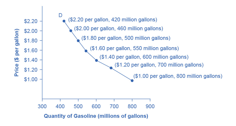
Figure 3.1: A Demand Curve for Gasoline
- At $1.00 per gallon, 800 million gallons are demanded.
- At $2.20 per gallon, only 420 million gallons are demanded.
Key Notes for Demand Curve
- Inverse Relationship: The demand curve shows an inverse relationship between price and quantity demanded. As price goes up, demand goes down, and as price goes down, demand goes up.
- Different Shapes: Demand curves can look different for different products. Some may be steep, others flat, some straight, and others curved. But they all slope downwards from left to right, showing the same basic relationship.
- Demand vs. Quantity Demanded: Demand is not the same as quantity demanded.
Demand: Refers to the relationship between different prices and the quantities demanded at those prices. It is illustrated by a demand curve or a demand schedule.
Quantity Demanded: Refers to a specific point on the demand curve or a specific quantity on the demand schedule.
By understanding demand schedules and curves, we can better grasp how prices affect the quantity of goods that people are willing to buy. This is a crucial concept in economics and helps us make sense of market behavior.
What is Supply?
Supply refers to the quantity of a good or service that producers are willing and able to sell at various prices over a given period. The supply curve shows the relationship between the price of a good and the quantity supplied.
Example: Imagine the farmer is growing wheat. If the price of wheat increases, the farmer is likely to grow more wheat to increase profits. This illustrates the law of supply: as the price of a good rises, the quantity supplied rises, and vice versa.
Factors Affecting Supply:
- Production Costs: Higher costs decrease supply.
- Technology: Improvements in technology can increase supply.
- Prices of Related Goods: The supply of a good can be affected by the prices of other goods.
- Expectations: If producers expect higher future prices, they might reduce supply now.
Graphing Supply Curves and Shifts
A supply curve slopes upward from left to right. An increase in supply shifts the curve to the right; a decrease shifts it to the left. In the textile industry, if a new, more efficient weaving machine is invented, the supply of textiles will increase, shifting the supply curve to the right.
Supply Schedule:
A supply schedule is a table that shows the quantity of a good or service that producers are willing and able to sell at various prices over a specific period. It lists different prices and the corresponding quantities supplied, illustrating the relationship between price and quantity supplied.
| Price (per gallon) | Quantity Supplied (millions of gallons) |
| $1.00 | 500 |
| $1.20 | 550 |
| $1.40 | 600 |
| $1.60 | 640 |
| $1.80 | 680 |
| $2.00 | 700 |
| $2.20 | 720 |
Table 3.2 Price and Supply of Gasoline
Supply Curve:
A supply curve is a graphical representation of the relationship between the price of a good or service and the quantity supplied. It is typically plotted with price on the vertical axis and quantity supplied on the horizontal axis. The supply curve generally slopes upward from left to right, indicating that higher prices lead to higher quantities supplied, reflecting the law of supply.
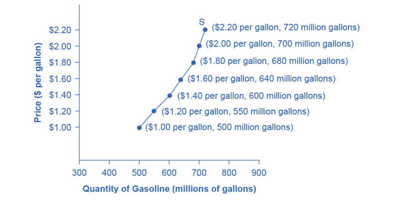
Figure 3.2: A Supply Curve for Gasoline
Key Notes for Supply Curve
- Direct Relationship: The supply curve shows a direct relationship between price and quantity supplied. As price goes up, supply goes up, and as price goes down, supply goes down.
- Different Shapes: Supply curves can look different for different products. Some may be steep, others flat, some straight, and others curved. But they all slope upwards from left to right, showing the same basic relationship.
- Supply vs. Quantity Supplied: Supply refers to the relationship between a range of prices and the quantities supplied at those prices. This can be illustrated with a supply curve or a supply schedule. Quantity supplied, on the other hand, refers to a specific point on the supply curve, or one quantity on the supply schedule. So, supply is about the entire curve, while quantity supplied is about a particular point on that curve.
Concept of Market
A market is a place or system where buyers and sellers interact to exchange goods, services, or resources. It can be physical (like a local farmers’ market) or virtual (like an online marketplace). Markets function based on the forces of supply and demand, determining the prices and quantities of goods and services exchanged.
Comparison of Perceived Demand and Market Demand
| Aspect | Perceived Demand | Market Demand |
| Definition | The demand curve as seen by an individual firm | The total demand for a product across the entire market |
| Relevance | Important for individual firm’s pricing and output decisions | Important for understanding the overall market behavior |
| Elasticity | Depends on the firm’s market power (e.g., perfect competition vs. monopoly) | Generally reflects the sum of individual consumer preferences |
| Shape in Perfect Competition | Horizontal (perfectly elastic) | Downward-sloping |
| Shape in Monopoly | Downward-sloping | Downward-sloping |
| Price Influence | Firm in perfect competition has no influence on price; a monopolist does | Determines the equilibrium price in the market |
| Quantity Influence | Firm adjusts quantity based on the given market price | Reflects total quantity demanded at various price levels |
| Examples | Individual farmer’s view in a wheat market | Total demand for wheat in the economy |
Explanation
Definition:
- Perceived Demand: The demand curve that an individual firm believes it faces. It can represent the suppliers’ or producers’ expectations to sell their products or services. For example, in perfect competition, a wheat farmer sees the price of wheat as given and can sell any quantity at that price.
- Market Demand: The total quantity of a product that all consumers in the market are willing to buy at various prices. It is the summation of all individual demands.
Relevance:
- Perceived Demand: Crucial for the firm’s decision-making about how much to produce and at what price to sell.
- Market Demand: Essential for understanding overall market trends, setting industry standards, and forming economic policies.
Elasticity:
- Perceived Demand: In perfect competition, the firm’s demand curve is perfectly elastic (horizontal), indicating that the firm can sell any amount at the market price. In a monopoly, the perceived demand curve is less elastic and downward-sloping.
- Market Demand: Reflects the overall price sensitivity of consumers. Generally, market demand curves slope downwards, indicating that lower prices lead to higher quantities demanded.
Shape in Perfect Competition:
- Perceived Demand: Horizontal, as firms are price takers and can sell any amount at the market price without affecting the price.
- Market Demand: Downward-sloping because, at higher prices, fewer people are willing or able to buy the product.
Shape in Monopoly:
- Perceived Demand: Downward-sloping as the monopolist can influence the market price by adjusting the quantity supplied.
- Market Demand: Also downward-sloping, representing the total demand in the market at various prices.
Price Influence:
- Perceived Demand: A perfectly competitive firm has no power to influence price and accepts the market price. A monopolist can set the price by choosing the quantity to produce.
- Market Demand: Determines the equilibrium price where total market supply equals total market demand.
Quantity Influence:
- Perceived Demand: An individual firm decides its production level based on the market price.
- Market Demand: Reflects the total amount of product demanded at different prices, which affects the overall production in the market.
Examples:
Perceived Demand:
- A wheat farmer in a perfectly competitive market.
- A utility company (e.g., electricity provider) in a monopolistic market.
Market Demand:
- Total demand for wheat across an entire country.
- Overall demand for electricity in a region.
Understanding these differences helps firms and policymakers make informed decisions about production, pricing, and market regulation.
The Ceteris Paribus Assumption
The Ceteris Paribus assumption is a fundamental concept in economics that simplifies the analysis of how one variable affects another. When economists look at how price influences the quantity demanded or supplied, they use this assumption to hold everything else constant. In other words, it means that they are examining the relationship between price and quantity without any interference from other factors. This allows for a clearer understanding of the cause-and-effect relationship between the two variables being studied. If other factors were allowed to change, it would be difficult to isolate the impact of price on quantity, and the usual laws of supply and demand might not apply. So, in simple terms, ceteris paribus means “assuming other factors being constant”.
Or “with all other things being the same” or “nothing else changes.”
Factors Affecting Demand and Shifts in Demand Curves
In economics, demand refers to the quantity of a product that consumers are willing and able to purchase at various prices. Several factors influence demand, leading to shifts in demand curves. Let’s explore these factors and their effects with real-world examples.
Factors Affecting Demand:
- Tastes and Preferences: Changes in consumer preferences impact demand. For example, if a new diet trend promotes healthier eating habits, the demand for organic foods might increase, while the demand for sugary snacks may decrease.
- Income: Income levels affect purchasing power. When income rises, consumers often buy more goods and services. Conversely, during economic downturns, lower income levels can lead to decreased demand. For instance, a rise in disposable income might increase the demand for luxury goods like high-end electronics or designer clothing. Disposable income is the amount of money that individuals have available for spending and saving after income taxes have been accounted for.
- Prices of Related Goods: The prices of substitutes and complements influence demand. Substitutes are products that can replace each other, such as tea and coffee. If the price of coffee increases, consumers may switch to tea, increasing the demand for tea. Complements are products used together, like Smartphones and data plans. A decrease in Smartphone prices may boost demand for data plans.
- Population Size and Composition: Changes in population demographics affect demand. For instance, an aging population may increase the demand for healthcare services and retirement homes. Similarly, an increase in the number of young families may boost the demand for childcare services and children’s products.
- Expectations: Consumer expectations about future prices or economic conditions can impact current demand. For example, if people anticipate a future price increase for gasoline due to geopolitical tensions, they may increase their current demand for gasoline to stock up before prices rise.
The Shift in Demand
Shifts in Demand Curves:
- Rightward Shift: An increase in demand shifts the demand curve to the right. This occurs when factors like rising incomes, changing preferences, or increased population lead to higher demand at every price level. For example, if a popular cooking show promotes the health benefits of olive oil, the demand for olive oil may increase, shifting the demand curve to the right.
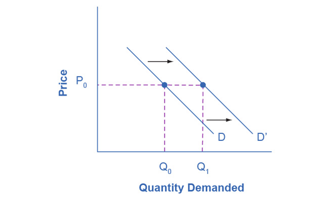
Figure 3.3 Demand Curve Shifted Right
- Leftward Shift: A decrease in demand shifts the demand curve to the left. Factors such as declining incomes, unfavorable trends, or shifts in preferences can cause lower demand at every price level. For instance, if concerns about environmental sustainability lead consumers to avoid products with excessive packaging, the demand for such products may decrease, shifting the demand curve to the left.

World Around Us: Shifts in Demand Curves
Let’s explore three real-world examples to illustrate factors affecting demand and shifts in demand curves:
Health-Conscious Food Choices:
You will better understand with an example about Tastes and Preferences.
Explanation: Changes in consumer preferences towards healthier food options can influence demand for certain products. As individuals become more health-conscious and prioritize nutritious eating habits, there is a shift in demand toward organic foods, plant-based alternatives, and functional beverages. Consumers are willing to pay premium prices for products perceived as healthier or environmentally sustainable.
Example: The increasing popularity of plant-based diets and awareness of sustainable farming practices have led to a surge in demand for plant-based meat substitutes, organic fruits and vegetables, and sustainably sourced food products. Companies like Beyond Meat and Impossible Foods have capitalized on this trend by offering plant-based burger patties and meat alternatives that appeal to health-conscious consumers seeking ethical and environmentally friendly food choices. This shift in consumer preferences has resulted in a notable increase in demand for plant-based products, prompting supermarkets and restaurants to expand their plant-based offerings and cater to evolving consumer tastes.
Home Exercise Equipment:
Changing Tastes or Preferences: The COVID-19 pandemic led to gym closures and increased emphasis on health and fitness, resulting in a surge in demand for home exercise equipment such as treadmills, stationary bikes, and dumbbells. Consumers sought alternatives to gym memberships and outdoor activities, driving up demand for home fitness solutions.
Income: Higher-income households may invest in high-end home exercise equipment with advanced features and capabilities. As incomes rise, the demand for premium home fitness products may increase, while lower-income consumers may opt for more affordable options or alternatives like resistance bands or bodyweight exercises.
Prices of Related Goods: The availability of online fitness classes or streaming platforms offering guided workouts can affect the demand for home exercise equipment. Lower prices for subscription services or bundled deals with equipment purchases may stimulate demand, especially if consumers perceive these services as valuable additions to their fitness routines.
Video Conferencing Software (e.g., Zoom, Microsoft Teams):
Changing Tastes or Preferences: The shift towards remote work and virtual meetings during the COVID-19 pandemic increased the demand for video conferencing software. Businesses, educational institutions, and individuals relied heavily on these platforms for communication and collaboration, leading to a significant rise in demand.
Income: Both businesses and individuals with stable incomes invested in video conferencing software to adapt to remote work and maintain communication channels. As remote work becomes more prevalent, the demand for video conferencing tools may remain high, especially among businesses willing to invest in premium features and services.
Prices of Related Goods: The availability of free or low-cost video conferencing solutions can affect the demand for premium software offerings. However, businesses and organizations may prioritize security, reliability, and additional features, leading to sustained demand for paid video conferencing platforms despite the availability of free alternatives.
The Shift in Demand with Income: Illustration with graph and table
Let’s use income as an example of how factors other than price affect demand. Figure 3.5 shows the initial demand for cars as D0. At point Q, if the price is $20,000 per car, the quantity demanded is 18 million. D0 also shows how the quantity demanded changes with different prices. For example, if the price of a car rises to $22,000, the quantity demanded decreases to 17 million, as shown at point R.
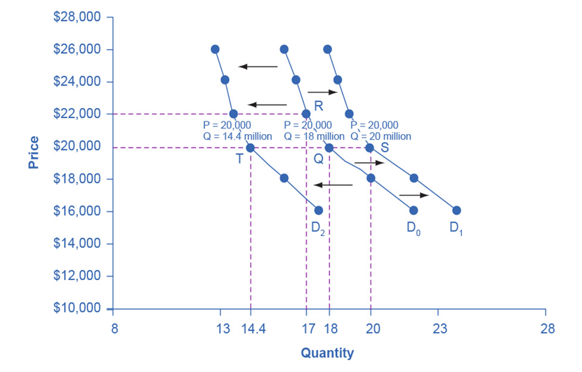
The original demand curve D0 assumes that no other factors change, following the ceteris paribus assumption. Now, imagine the economy improving, increasing many people’s incomes, and making cars more affordable. How will this affect demand?
Refer to Figure 3.5. The price of cars remains $20,000, but with higher incomes, the quantity demanded increases to 20 million cars, shown at point S. As a result, the demand curve shifts to the right to D1, indicating higher demand. Table 3.4 shows that this increased demand occurs at every price, not just the original one.
The graph shows the original demand curve D0, the increased income demand curve D1, and the decreased income demand curve D2. Increased demand means at every price, the quantity demanded is higher, shifting the demand curve right from D0 to D1. Decreased demand means at every price, the quantity demanded is lower, shifting the demand curve left from D0 to D2.
Now, imagine the economy slowing down, causing job losses or reduced working hours, lowering incomes. This would lead to a lower quantity of cars demanded at every price, shifting the original demand curve D0 left to D2. At $20,000, 18 million cars are sold on the original curve, but only 14.4 million after the demand decreases.
| Price | Decrease to D2 | Original Quantity Demanded D0 | Increase to D1 |
| $16,000 | 17.6 million | 22.0 million | 24.0 million |
| $18,000 | 16.0 million | 20.0 million | 22.0 million |
| $20,000 | 14.4 million | 18.0 million | 20.0 million |
| $22,000 | 13.6 million | 17.0 million | 19.0 million |
| $24,000 | 13.2 million | 16.5 million | 18.5 million |
| $26,000 | 12.8 million | 16.0 million | 18.0 million |
Table 3.4 Price and Demand Shifts: A Car Example
A shift in the demand curve doesn’t mean every individual’s demand changes equally. Not everyone will experience the same income changes or buy the same amount of cars. Instead, it shows a market-wide pattern.
Points to Remember:
We previously noted that higher income usually increases demand at every price. This is true for most goods and services. For some items like luxury cars, European vacations, and fine jewelry, the demand increases with higher income can be more significant. These are called normal goods. However, some goods, like generic groceries, used cars, and rental housing, see decreased demand as incomes rise. These are called inferior goods, and their demand curve shifts left when incomes rise.
Understanding these factors and shifts in demand curves helps businesses and policymakers anticipate changes in consumer behavior and make informed decisions about pricing, production, and resource allocation. By analyzing real-world examples within the framework of demand theory, economists can provide valuable insights into market dynamics and trends.
Equilibrium, Changes in Equilibrium Price and Quantity: The Four-Step Process
Identifying Equilibrium Price and Quantity:
The equilibrium price and quantity are determined where the demand and supply curves intersect. At this point, the quantity demanded equals the quantity supplied.
Example: Consider the market for tea in Bangladesh. If the price of tea is too high, there will be a surplus (more tea than people want to buy). If the price is too low, there will be a shortage (not enough tea to meet demand). The equilibrium price is where these two forces balance out.
The Four-Step Process to Reach Equilibrium:
- Draw the Demand and Supply Curves: Identify the initial equilibrium price and quantity, the intersection points of demand and supply curves.
- Determine the Shift: Identify whether the change in price or change in quantity affects demand or supply.
- Shift the Curve: Show how the demand or supply curve shifts.
- Find the New Equilibrium: Determine the new equilibrium price and quantity.
Let’s use the example of gasoline to understand how demand and supply interact. We can illustrate this with a graph showing both the demand curve and the supply curve for gasoline.
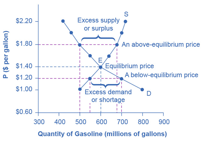
Figure 3.6: Demand and Supply for Gasoline
The demand curve (D) slopes downward, indicating that as the price of gasoline decreases, and the quantity demanded increases. The supply curve (S) slopes upward, showing that as the price increases, the quantity supplied also increases. These curves intersect at the equilibrium point (E), which, in our example, is at a price of $1.40 per gallon and a quantity of 600 million gallons.
| Price (per gallon) | Quantity Demanded (millions of gallons) | Quantity Supplied (millions of gallons) |
| $1.00 | 800 | 500 |
| $1.20 | 700 | 550 |
| $1.40 | 600 | 600 |
| $1.60 | 550 | 640 |
| $1.80 | 500 | 680 |
| $2.00 | 460 | 700 |
| $2.20 | 420 | 720 |
Table 3.3: Price, Quantity Demanded, and Quantity Supplied
Finding the Equilibrium
The equilibrium price is where the quantity demanded equals the quantity supplied. In our gasoline example, this is $1.40 per gallon, with 600 million gallons demanded and supplied.
If you only had the demand and supply schedules (like Table 3.3) and not the graph, you could still find the equilibrium by looking for the price where the quantity demanded equals the quantity supplied.
Price above Equilibrium
What happens if the price is above the equilibrium price? For example, if gasoline is priced at $1.80 per gallon:
- The quantity demanded drops to 500 million gallons because consumers react to higher prices by using less gasoline.
- The quantity supplied increases to 680 million gallons because producers are motivated by higher prices to produce more.
- There is an excess supply (or surplus) of 180 million gallons (680 supplied – 500 demanded).
With a surplus, gasoline accumulates at various stages of distribution. This accumulation puts pressure on sellers to lower prices to sell off the excess. As prices decrease, the quantity demanded will increase, moving the market back towards equilibrium.
Price below Equilibrium
Conversely, if the price is below the equilibrium price, for example at $1.20 per gallon:
- The quantity demanded increases to 700 million gallons as lower prices encourage more consumption.
- The quantity supplied decreases to 550 million gallons because producers are less motivated to supply at lower prices.
- There is an excess demand (or shortage) of 150 million gallons (700 demanded – 550 supplied).
With a shortage, consumers will find gasoline in short supply and will be willing to pay higher prices. This increased willingness to pay leads sellers to raise prices, moving the market back towards equilibrium.
Key Notes for Equilibrium
- Equilibrium Price: The price at which quantity demanded equals quantity supplied.
- Surplus: Occurs when the price is above equilibrium, leading to excess supply.
- Shortage: Occurs when the price is below equilibrium, leading to excess demand.
- Market Forces: Surpluses and shortages create pressures referred to as market forces that move the price towards the equilibrium.
World Around Us: Equilibrium
Market for Fresh Vegetables
Scenario: During the harvest season, farmers bring a large supply of fresh vegetables to the market.
High Supply: Farmers have an abundant supply of vegetables.
Demand Response: Consumers are willing to buy more vegetables if the price is reasonable.
Equilibrium:
- Initial Price: If the price is too high, consumers will not buy all the vegetables, leading to excess supply.
- Adjustment: Farmers reduce prices to sell their produce.
- New Equilibrium: The price drops to a point where consumers buy all the vegetables, and there is no surplus. For instance, if the price per kilogram drops from $3 to $2, and the quantity demanded increases to match the quantity supplied, equilibrium is achieved.
Housing Market
Scenario: A city experiences an influx of new residents due to a booming job market.
High Demand: More people want to rent or buy homes.
Limited Supply: The number of available homes remains the same in the short term.
Equilibrium:
- Initial Price: If the rent or price of homes is initially low, the increased demand will lead to a shortage.
- Adjustment: Landlords and sellers raise prices because more people are competing for the same number of homes.
- New Equilibrium: Prices rise until they reach a level where the quantity of homes demanded equals the quantity supplied. For example, if the monthly rent increases from $1,000 to $1,500, the demand may decrease as some people opt for different housing options or locations, balancing the market.
Market for Smartphone
Scenario: A new Smartphone model is released, and it becomes very popular.
High Demand: Consumers rush to buy the new Smartphone.
Limited Initial Supply: The manufacturer has a limited number of units available at launch.
Equilibrium:
- Initial Price: If the price is set too low, the Smartphones sell out quickly, leading to a shortage.
- Adjustment: Seeing the high demand, the manufacturer or retailers might raise the price.
- New Equilibrium: The price increases until it reaches a point where the quantity of Smartphones demanded equals the quantity supplied. For example, if the price rises from $700 to $900, demand might decrease as some consumers decide to wait or buy alternative models, leading to equilibrium.
*Task: Collect data for these examples from different available sources to you. Draw demand and supply curves and find equilibriums for the above examples.
Understanding these concepts helps explain how markets function and how prices are determined in real-world situations. For instance, when a natural disaster affects oil production, it can shift the supply curve, leading to higher prices and changes in quantity demanded and supplied. Similarly, technological advancements can shift the supply curve, lowering prices and increasing the quantity supplied.
Price Controls, Price Ceilings, and Price Floors: A Simplified Explanation
Price Controls: Price controls are regulations set by the government to manage the cost of goods and services in a market. These controls come in two main forms: price ceilings and price floors.
Price Ceilings:
A price ceiling is a legal maximum price for a product. It’s designed to prevent prices from rising too high, ensuring essential goods remain affordable.
World Around Us: Price Ceilings
Pharmaceutical Price Controls in Canada
Example: The Canadian government enforces price ceilings on many prescription drugs to ensure they remain affordable for citizens. The Patented Medicine Prices Review Board (PMPRB) regulates the maximum price that can be charged for patented medicines in Canada.
Impact: These price controls help keep drug prices significantly lower than in neighboring countries like the United States. While this makes medications more accessible to Canadians, it can also lead to drug shortages and reduced incentives for pharmaceutical companies to introduce new drugs in Canada.
Gasoline Price Caps in Venezuela
Example: The government of Venezuela has imposed price ceilings on gasoline for many years to make it affordable for the public. The price of gasoline in Venezuela has been among the lowest in the world due to these controls. The government of Venezuela has a long history of imposing price ceilings on gasoline. The practice dates back to the 1950s and was particularly emphasized during the presidency of Hugo Chavez, who began his term in 1998 Gasoline prices in Venezuela have indeed been among the lowest in the world, averaging around 0.02 USD/Liter from 2020 to 20242.
Impact:
While this policy makes gasoline very cheap for consumers, it has led to significant negative consequences. These include severe shortages, long lines at gas stations, and a thriving black market where gasoline is sold at much higher prices. The artificially low prices have also contributed to the economic crisis by reducing the revenues needed to maintain and invest in the oil industry.
Food Price Ceilings in Zimbabwe
Example: During periods of economic instability and hyperinflation, the Zimbabwean government has imposed price ceilings on basic food items like bread, maize meal, and cooking oil to make them affordable for the population. The use of price controls in Zimbabwe has often coincided with episodes of hyperinflation, particularly during the late 2000s when the country experienced extreme economic challenges. For example, in 2007, the government ordered prices to be halved on many commodities, leading to widespread shortages.
More recently, the government has continued to grapple with economic challenges, including inflation and currency issues. In 2019, the government reintroduced the Zimbabwean dollar (ZWL) and has since been managing the pricing of essential goods to prevent runaway inflation and ensure affordability for its citizens
Impact:
These price controls often lead to severe shortages of these essential goods. Producers and retailers, unable to cover their costs due to the low prices, reduce production or stop selling these items altogether. This results in empty shelves in stores and long queues for basic foodstuffs. Additionally, it encourages the development of black markets where these goods are sold at much higher prices.
Graphical Illustration of Price Ceiling
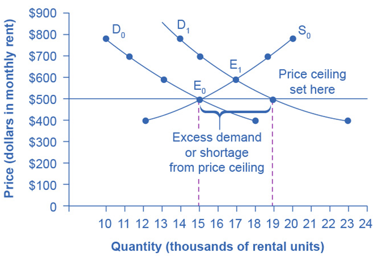
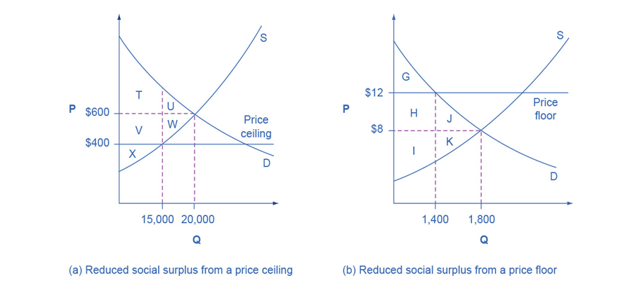
In cities like New York, Washington D.C., and San Francisco, rent control laws limit how much landlords can increase rent annually. If a city passes a law to keep rent at $500 per month when the market price rises to $600 due to higher demand, a shortage occurs. More people want to rent at a lower price (19,000 units), but fewer units (15,000) are available, resulting in a shortage of 4,000 units. While rent control aims to make housing affordable, it often leads to fewer available units and lower quality of maintenance.
Rent control can cause several issues. Since landlords can’t charge higher rents, they might not have enough money to properly maintain the property. This can lead to apartments becoming run-down over time. Also, with the limited number of units available, finding a place to rent becomes harder for new tenants. In summary, while rent control is intended to help tenants by keeping rents low, it can result in fewer available apartments and poorer living conditions.
| Price | Original Quantity Supplied | Original Quantity Demanded | New Quantity Demanded |
| $400 | 12,000 | 18,000 | 23,000 |
| $500 | 15,000 | 15,000 | 19,000 |
| $600 | 17,000 | 13,000 | 17,000 |
| $700 | 19,000 | 11,000 | 15,000 |
| $800 | 20,000 | 10,000 | 14,000 |
Table 3.7 Rent Control
Price Floors
A price floor sets a minimum price for a product, ensuring it doesn’t fall too low. The minimum wage is a common example. The federal minimum wage in 2022 in USA was $7.25 per hour, aimed at ensuring workers can afford basic living standards. Similarly, agricultural price supports are another form of price floor. Governments buy up surplus crops to keep prices high, helping farmers maintain stable incomes. For instance, the European Union spends billions on such support to prevent farm incomes from dropping during bad years.
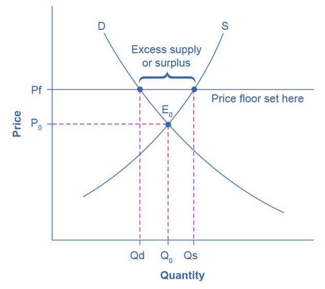
In the wheat market in Europe, if the government sets a price floor above the equilibrium price, it creates a surplus. Farmers produce more wheat than consumers buy at this higher price, and the government must buy the excess. This benefits farmers but costs taxpayers and can distort the market. You will better understand with the following examples.
World Around Us: Price Floors
Sugar Price Supports in the United States
- The U.S. government maintains a minimum price for sugar by implementing loan programs and marketing allotments. Farmers receive loans from the government with sugar as collateral. If market prices fall below the loan rates, farmers can surrender their sugar to the government to satisfy the loan, effectively setting a price floor.
- The government also controls the amount of sugar that can be sold domestically, limiting supply to keep prices above a certain level.
Impacts:
- Consumer Impact: Consumers face higher prices for sugar and sugar-containing products compared to what they would pay in a free market. This increase in price can affect both individual consumers and food manufacturers, potentially leading to higher overall food prices.
- Producer Impact: Domestic sugar producers benefit from stable and higher prices, which ensures their income remains consistent. This support helps them survive against international competition where sugar might be produced more cheaply.
- Market Impact: Overproduction can occur because producers are guaranteed a higher price, leading to surplus sugar that the government must buy or store, increasing government expenditure.
- International Trade: Higher domestic prices can lead to tensions with other sugar-producing countries and affect trade policies, possibly resulting in retaliatory tariffs or trade disputes.
Alcohol Minimum Pricing in Scotland
- The minimum unit pricing (MUP) policy in Scotland sets a minimum price per unit of alcohol. For example, if the MUP is set at 50 pence per unit, a bottle of wine containing 10 units of alcohol cannot be sold for less than £5.
- The policy aims to reduce alcohol consumption by making it more expensive, particularly targeting cheap and high-strength alcoholic beverages.
Impacts:
- Public Health Impact: The primary goal is to reduce alcohol-related harm, including health issues, crime, and social problems. Early studies suggest that MUP has led to a reduction in alcohol sales and a drop in alcohol-related hospital admissions.
- Consumer Impact: While the policy benefits public health, it also increases the cost of alcohol for consumers, particularly affecting those who consume large quantities of cheap alcohol. Moderate drinkers buying more expensive brands might see less of an impact.
- Retailer Impact: Retailers may experience a decrease in sales of cheaper alcoholic products but could see a shift towards higher-priced options. Smaller retailers relying on sales of cheap alcohol might be more adversely affected.
- Economic Impact: The policy could potentially reduce government spending on health care and law enforcement related to alcohol abuse. However, it might also reduce overall consumer spending in the economy as people allocate more of their budget to alcohol.
Dairy Price Support Programs in the European Union
- The EU supports dairy prices through intervention buying and quotas. The government buys dairy products like butter and powdered milk if market prices fall below a certain threshold ensuring farmers receive a minimum price.
- Production quotas limit the amount of milk that can be produced to prevent market oversupply.
Impacts:
- Producer Impact: Dairy farmers receive stable and predictable income, which helps them manage production costs and invest in their farms. This support is particularly crucial for smaller farms that might struggle with volatile prices.
- Consumer Impact: Consumers may face higher prices for dairy products than they would in a free market. This increase can affect household budgets, particularly in lower-income households.
- Market Impact: Government intervention can lead to inefficiencies, such as overproduction. Surplus products may need to be stored or sold at a loss, leading to additional costs for the government and taxpayers.
- Environmental Impact: Price supports can encourage overproduction, which might lead to environmental issues like overgrazing, increased greenhouse gas emissions, and higher use of water and land resources.
- Trade Impact: The policy can affect international trade relationships. Non-EU countries may face barriers when exporting their dairy products to the EU, leading to trade imbalances and potential disputes.
Key Points for Price Control Mechanism
- Price controls are government regulations to manage the cost of goods.
- Price ceilings cap prices to keep them from rising too high, but can lead to shortages and lower quality.
- Price floors set minimum prices to prevent them from falling too low, creating surpluses that the government often buys up to support producers.
- Price ceilings can make essential goods and services more affordable.
- However, they often lead to shortages and unintended market distortions.
- These policies can create black markets and reduce the quality and availability of goods.
- Price floors can help ensure fair wages and stabilize incomes for producers.
- Price floors also lead to surpluses, inefficiencies, and higher costs for consumers and taxpayers.
- Price floors might achieve social goals, such as reducing harmful behaviors, but they can also have unintended economic consequences.
Consumer Surplus, Producer Surplus, and Social Surplus
Consumer Surplus:
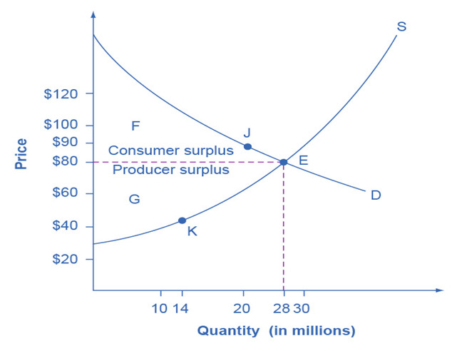
This is the benefit consumers get when they pay less for a product than what they are willing to pay. For instance, if someone is willing to pay $90 for a tablet but buys it for $80, they enjoy a $10 surplus. In a market, consumer surplus is shown as the area above the equilibrium price and below the demand curve.
Producer Surplus
This is the benefit producers get when they sell a product for more than what they are willing to accept. For example, if a producer is willing to sell a tablet for $45 but sells it for $80, they gain a $35 surplus. In a market, producer surplus is shown as the area below the equilibrium price and above the supply curve.
Social Surplus:
This is the total benefit to society, combining both consumer and producer surpluses. It is maximized at the market equilibrium, where the amount of goods supplied equals the amount of goods demanded. Social surplus represents the overall economic efficiency in the market.
World Around Us
Consumer Surplus Examples
Example 1: Online Shopping Deals
- Scenario: A consumer finds a high-quality pair of headphones online for $100, but they are willing to pay up to $150.
- Consumer Surplus: The difference, $50, represents the consumer surplus.
- Benefits: Consumers feel they are getting a good deal, which can increase customer satisfaction and loyalty.
- Drawbacks: If the price is consistently low, it might lead to an unsustainable market where producers cannot maintain profits.
Example 2: Airline Tickets
- Scenario: A passenger is willing to pay $500 for a flight but finds a ticket for $300 during a sale.
- Consumer Surplus: The consumer surplus is $200.
- Benefits: Sales and discounts can make travel more accessible to more people.
- Drawbacks: Airlines might reduce the quality of service or charge extra fees to compensate for the lower ticket prices.
Example 3: Seasonal Sales
- Scenario: During a Black Friday sale, a consumer buys a TV for $400 that they were willing to pay $600 for.
- Consumer Surplus: The surplus here is $200.
- Benefits: Seasonal sales boost consumer purchasing power, allowing them to buy more with the same amount of money.
- Drawbacks: Retailers may struggle with reduced profit margins and might need to compensate by cutting costs elsewhere.
Producer Surplus Examples
Example 1: Farmer’s Market
- Scenario: A farmer is willing to sell apples for $1 per pound but sells them for $2 per pound at a farmer’s market.
- Producer Surplus: The surplus is $1 per pound.
- Benefits: Producers can reinvest this extra profit into their business, improving quality and expanding production.
- Drawbacks: Higher prices might reduce the number of buyers, potentially lowering overall sales volume.
Example 2: Technology Products
- Scenario: A tech company develops a new gadget and is willing to sell it for $200 but finds that the market price is $300.
- Producer Surplus: The producer surplus is $100.
- Benefits: High profits can drive innovation and further research and development.
- Drawbacks: High prices may limit access to the product, making it affordable only for wealthier consumers.
Example 3: Art and Collectibles
- Scenario: An artist is willing to sell a painting for $1,000, but it sells at an auction for $10,000.
- Producer Surplus: The producer surplus here is $9,000.
- Benefits: The artist gains significant financial rewards, which can support their career and future projects.
- Drawbacks: High prices can create exclusivity, limiting the appreciation of art to a small, affluent segment of the population.
Benefits and Drawbacks of Surplus
Benefits of Consumer Surplus
- Increased Consumer Welfare: Consumers get more value than what they pay for.
- Higher Purchasing Power: Surplus allows consumers to buy more or save money for other uses.
- Market Efficiency: Indicates that consumers are receiving goods at prices they value more highly than the cost.
Drawbacks of Consumer Surplus
- Producer Strain: Consistently low prices might pressure producers, leading to lower quality or business closures.
- Unsustainable Practices: If prices are driven too low, it can result in unsustainable production practices.
Benefits of Producer Surplus
- Incentive for Production: A high surplus motivates producers to continue and expand production.
- Economic Growth: Producers can reinvest surplus profits into their businesses, driving economic growth.
- Innovation: Extra profits provide capital for research and development, fostering innovation.
Drawbacks of Producer Surplus
- Consumer Access: High prices can limit access to goods and services for some consumers.
- Market Inequality: A significant producer surplus can contribute to wealth inequality.
- Potential for Monopolies: High profits might lead to monopolistic practices, reducing competition in the market.
In summary, consumer and producer surpluses reflect the benefits that different market participants receive. While they offer significant advantages, such as increased welfare and incentives for production, they also come with drawbacks like market imbalances and potential sustainability issues.
Inefficiency of Price Floors and Price Ceilings
Price Ceilings:
A price ceiling is the maximum price set by the government for a product, preventing it from rising above this limit. An example is rent control, which sets the maximum rent landlords can charge. While intended to help renters, it often leads to shortages as the quantity demanded exceeds the quantity supplied. This inefficiency creates a deadweight loss, meaning some potential gains from trade are lost. Additionally, some producer surplus is transferred to consumers, but overall, social surplus decreases.
Price Floors:
A price floor is a minimum price set by the government for a product, preventing it from the falling below this limit. An example is the minimum wage, which sets the lowest amount a worker can be paid per hour. While intended to help workers, it can lead to surpluses as the quantity supplied exceeds the quantity demanded, like in the case of excess labor leading to unemployment. This also creates a deadweight loss and reduces overall social surplus. Some consumer surplus is transferred to producers, but the market becomes less efficient. The benefit to consumers is smaller than the loss to producers, which illustrates the deadweight loss.
Demand and Supply as a Social Adjustment Mechanism
Market Dynamics:
Prices in a market are determined by the interaction of demand and supply. Economist Alfred Marshall compared it to both blades of scissors working together to cut paper. Prices adjust based on changes in demand and supply without the need for government intervention.
If a frost in Brazil reduces the coffee supply, the supply curve shifts left, and prices rise. Consumers might switch to tea or soft drinks, and this adjustment happens naturally in the market.
Seasonal foods like fresh corn are cheaper in midsummer when supply is high. People adjust their diets and restaurants change menus based on these price changes, demonstrating the market’s role in efficiently allocating resources.
Conclusion
Efficiency in Markets:
When markets operate without intervention, they tend to be efficient, maximizing social surplus by ensuring that goods and services are produced and consumed in optimal quantities.
Impact of Price Controls:
Price floors and ceilings disrupt this efficiency, creating shortages or surpluses and leading to deadweight loss. While they might benefit specific groups (renters or workers), they generally reduce the overall economic benefit to society.
Example: In agriculture, if there is a bumper crop of rice in India, the increased supply will lower prices, signaling farmers to plant less rice the next season or shift to other crops.
Deadweight Loss
Deadweight loss refers to the loss of economic efficiency (or the loss of social surplus) that occurs when the equilibrium for a good or service is not achieved or is not achievable. It represents the loss of potential gains from trade that neither consumers nor producers can capture. This inefficiency often results from market distortions such as taxes, subsidies, price ceilings, or price floors. Hence deadweight loss is the reduction in total economic welfare that occurs when the economy produces a quantity of goods or services that is not at the optimal level.
Summary
Understanding demand and supply is fundamental to analyzing how markets operate. By recognizing how various factors shift demand and supply, and how these shifts affect equilibrium, we can better comprehend market dynamics. Whether at the individual, firm, or national level, these concepts help us make informed decisions and understand economic phenomena in our everyday lives.
Case Study: Demand and Supply through the Lens of Behavioral Economics
Traditional economics assumes that people respond to changes in demand and supply rationally. For example, when prices rise, demand falls, and when prices fall, demand rises. However, behavioral economics suggests that human behavior often deviates from this rational model due to psychological influences.
Scenario: Consumer Response to Price Changes
Imagine a situation where the price of a popular smartphone suddenly drops due to a new model being released. Traditional economics would expect a sharp increase in demand for the older model because it’s now cheaper. But, behavioral economics shows that the actual response might be different.
Cognitive Biases
- Anchoring Bias: Consumers might anchor their perception of the smartphone’s value based on its original, higher price. Even with a price drop, some might still see it as too expensive compared to other options.
- Confirmation Bias: Consumers who believe that newer is always better may ignore the price drop and opt for the newer model, even if the older one offers better value.
Prospect Theory and Loss Aversion
- Loss Aversion: Some consumers might avoid buying the discounted smartphone because they fear missing out on the latest features of the new model. They see this as a potential “loss” even though the older model might meet their needs perfectly.
- Framing Effect: If the price drop is framed as a “clearance sale,” consumers might perceive the product as less valuable or outdated, reducing demand despite the lower price.
Heuristics
- Availability Heuristic: Consumers might overestimate the importance of the latest smartphone based on recent advertisements or news, leading them to ignore the older model’s price drop.
Nudging
- Nudge: Retailers could nudge consumers by offering limited-time discounts or bundling the older model with accessories to increase its appeal. This could shift demand in favor of the discounted product.
Time Inconsistency
- Present Bias: Consumers might prioritize immediate gratification and choose the newer, more expensive model, believing it will make them happier now, even if the older model is more practical.
Impact and Analysis
Behavioral economics helps us understand why consumer demand doesn’t always rise as expected when prices fall. Psychological factors like biases, loss aversion, and the framing of choices play a significant role in how people respond to changes in supply and demand.
References
- Thaler, R. H., & Sunstein, C. R. (2008). Nudge: Improving Decisions About Health, Wealth, and Happiness.
- Kahneman, D. (2011). Thinking, Fast and Slow.
- Tversky, A., & Kahneman, D. (1979). Prospect Theory: An Analysis of Decision under Risk.
Research Suggestions for Economists in the Context of Behavioral Economics
Behavioral Determinants of Price Elasticity
- Objective: Investigate how cognitive biases, such as loss aversion or anchoring, influence consumer price sensitivity and the elasticity of demand for different products.
- Methodology: Conduct experiments or surveys where consumers make purchasing decisions under varying price scenarios. Analyze how their price elasticity deviates from traditional models due to behavioral factors.
- Expected Outcome: Identify specific biases that cause deviations in price elasticity and suggest models that integrate these behavioral insights.
Impact of Behavioral Nudges on Demand Patterns
- Objective: Explore how behavioral nudges, like default options or framing effects, can shift consumer demand towards more sustainable or healthier products.
- Methodology: Implement nudges in retail environments or online platforms, such as highlighting healthier food choices or setting energy-efficient products as the default. Measure the changes in demand patterns before and after the intervention.
- Expected Outcome: Provide empirical evidence on the effectiveness of nudges in altering demand and suggest policy implications for influencing consumer behavior.
Time Inconsistency in Consumer Demand
- Objective: Study how time-inconsistent preferences, where consumers prioritize short-term gratification over long-term benefits, affect demand for products like savings plans, insurance, or luxury goods.
- Methodology: Use longitudinal studies or experiments where consumers make choices between immediate rewards and delayed benefits. Analyze how their demand for different products changes over time.
- Expected Outcome: Offer insights into how time inconsistency impacts market demand and suggest strategies for firms or policymakers to address these behavioral tendencies.
Behavioral Economics of Supply Chain Decisions
- Objective: Investigate how biases like overconfidence or herd behavior influence supply chain decisions, particularly in inventory management and production planning.
- Methodology: Conduct case studies or simulations where supply chain managers must make decisions under uncertainty. Assess how their decisions deviate from rational models due to behavioral factors.
- Expected Outcome: Identify common behavioral pitfalls in supply chain management and propose interventions to improve decision-making efficiency.
Social Influence and Demand Fluctuations
- Objective: Examine how social factors, such as peer pressure or social norms, impact consumer demand for products, especially in markets driven by trends (e.g., fashion, technology).
- Methodology: Use social media data, surveys, or experiments to analyze how social influences lead to shifts in demand. Compare these findings with traditional demand models.
- Expected Outcome: Highlight the role of social influence in creating demand surges or slumps, and suggest ways to incorporate these factors into demand forecasting.
Heuristics in Market Supply Decisions
- Objective: Study how heuristics, like the availability heuristic or representativeness, influence supply decisions made by producers, particularly in markets with fluctuating demand.
- Methodology: Design experiments or surveys where producers must make supply decisions based on limited information. Assess how their reliance on heuristics affects market supply outcomes.
- Expected Outcome: Provide insights into how heuristics can lead to overproduction or underproduction, and suggest strategies for reducing these effects in supply planning.
These research suggestions aim to bridge the gap between traditional demand and supply models and the behavioral tendencies that influence real-world economic decisions. Integrating behavioral economics into these areas can lead to a more comprehensive understanding of market dynamics and inform more effective economic policies and business strategies.
Critical Thinking
- How would a major technological advancement in the production of electric cars impact the supply and demand curves for electric cars? Discuss the short-term and long-term effects on equilibrium price and quantity.
- Discuss the potential unintended consequences of implementing a price ceiling on essential goods like pharmaceuticals. What might happen to the quality and availability of these goods in the market?
- Analyze how a significant increase in the price of gasoline might affect the demand for electric vehicles and public transportation. Consider the roles of substitute and complementary goods in your analysis.
- What are some examples of external shocks that can disrupt market equilibrium? Choose an example and explain how the supply and demand curves might shift as a result.
- Suppose the government provides a subsidy to producers of solar panels to encourage clean energy use. How would this subsidy affect the supply curve for solar panels? Discuss the likely changes in equilibrium price and quantity. What might be some unintended consequences of this subsidy?
- Analyze how a natural disaster, such as a hurricane, affects the supply and demand for building materials like lumber and concrete. What are the short-term and long-term impacts on prices and quantities in the affected market?
- Evaluate the effectiveness of rent control policies in keeping housing affordable for low-income residents. What are the potential unintended consequences of rent control on the availability and quality of rental housing?
- Consider a market where a significant technological innovation reduces production costs for a particular good, such as 3D printing technology for manufacturing. How does this innovation affect the supply curve, equilibrium price, and quantity in the market?Discuss how global supply chain disruptions, like those caused by a pandemic, impact the supply and demand for goods such as medical supplies or consumer electronics.
- What strategies can businesses and governments use to mitigate these disruptions?
- Analyze how a cultural shift towards healthier eating habits might impact the demand for fast food versus organic food products. How would these changes affect the respective markets in terms of prices and quantities?
- Discuss how seasonal variations affect the demand and supply for products such as holiday decorations or winter clothing. How do businesses plan for these variations, and what strategies do they use to manage inventory and pricing?

